Inference for proportions

STA 101L - Summer I 2022

Raphael Morsomme

Welcome

Announcements

Data analysis in action – Inferring ethnicity from X-rays
Anonymous mid-course feedback

Recap

Statistical inference
Five cases
Hypothesis test
Confidence interval
A first glimpse of modern statistics

Outline

One proportion (case 1)
Two proportions (case 2)

One proportion

Setup

population parameter: proportion \(p\)

Sample statistics: sample proportion \(\hat{p}\)

Hypothesis testing:

\(H_0:p=p_0\) where \(p_0\) is a number between \(0\) and \(1\)
\(H_a:p\neq p_0\)

Confidence interval: range of plausible values for \(p\).

One-sided and two-sided \(H_a\)

One-sided) \(H_a:p>p_0\) or \(H_a:p<p_0\)

Two-sided) \(H_a: p\neq p_0\)

It is never wrong to use a two-sided \(H_a\).

Individual exercise - Hypotheses

Exercise 16.1

01:00

Example – legalizing marijuana

What proportion of US adults support legalizing marijuana?

Sample: 900/1500 support it.

\[ \hat{p} = \dfrac{900}{1500}=0.6 \]

Hypothesis test via simulation

\(H_0:p=0.5\)

\(H_a:p\neq 0.5\)

Simulate many samples under \(H_0\).
Determine if the observed data could have plausibly arisen under \(H_0\).

Parametric bootstrap

The textbook uses the term (parametric) bootstrap to refer to this procedure.

set.seed(0)
results <-  tibble(p_hat = numeric())
for(i in 1 : 1e4){
  sim     <- rbernoulli(n = 1500, p = 0.5) # simulate a sample under H0
  p_hat   <- mean(sim)                     # compute the sample statistic p_hat
  results <- results %>% add_row(p_hat = p_hat)
}
ggplot(results) + geom_histogram(aes(p_hat))

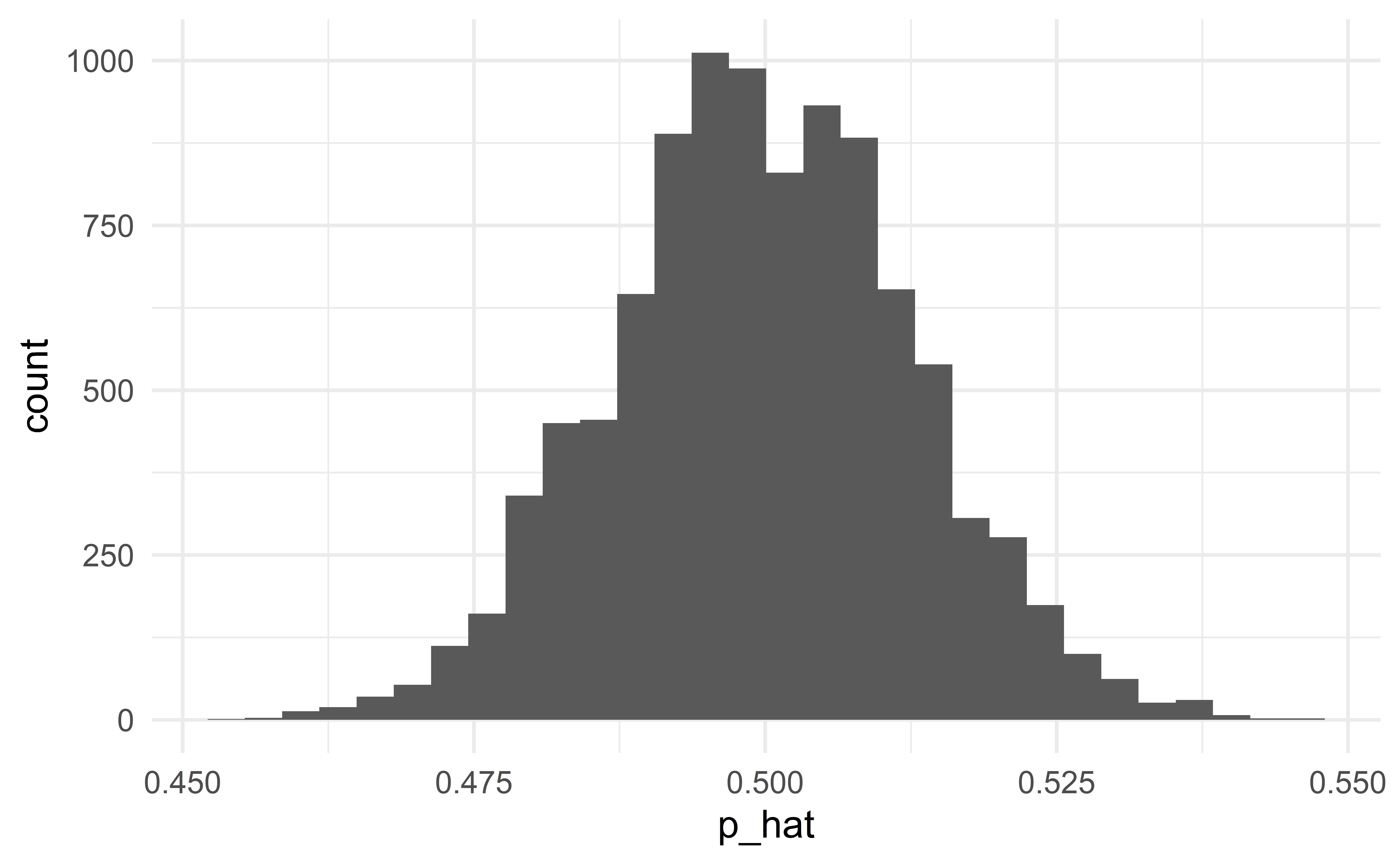
Conclusion

\(\hat{p}=0.6\) is extremely unlikely to happen under \(H_0:p=0.5\).

We therefore reject the null hypothesis that half of the people support legalizing marijuana.

Group exercise - HT for one proportion

Exercise 16.3 – in part d, you do not need to estimate the p-value.

03:00

p-value

What if we do not have a clear-cut case?

e.g., \(\hat{p}=0.52 = \dfrac{780}{1500}\)

p-value: probability that the sample statistic of a sample simulated under \(H_0\) is at least as extreme as that of the observed sample.

the probability that \(\hat{p}_{sim} > 0.52\) or \(\hat{p}_{sim} < 0.48\).

p-value in `R`

results <- results %>%
  mutate(is_more_extreme = p_hat <= 0.48 | p_hat >= 0.52)
results

# A tibble: 10,000 x 2
   p_hat is_more_extreme
   <dbl> <lgl>          
 1 0.475 TRUE           
 2 0.485 FALSE          
 3 0.483 FALSE          
 4 0.528 TRUE           
 5 0.51  FALSE          
 6 0.493 FALSE          
 7 0.503 FALSE          
 8 0.5   FALSE          
 9 0.495 FALSE          
10 0.503 FALSE          
# ... with 9,990 more rows

results %>% summarize(p_value = mean(is_more_extreme))

# A tibble: 1 x 1
  p_value
    <dbl>
1   0.127

p-value in practice

In practice, if a p-value is smaller than 0.05 we reject \(H_0\)

\(\alpha = 0.05\) is called the significance level.
If \(p<0.05\), the observed sample is in the top 5% of the most extreme simulated samples.
It is highly unlikely that the observed sample could have arisen if \(H_0\) were true.
the difference \(\hat{p}-p_0\) is statistically significant.

Why \(\alpha = 0.05\)?

To know why the significance level 0.05 is widely used in practice, check out this short video.

Group exercise - HT for one proportion

Exercise 16.5.

04:00

Confidence interval via bootstrap

Bootstrapping

Sample with repetition from the observed sample to construct many bootstrap samples.

Bootstrap samples \(\Rightarrow\) sampling distribution \(\Rightarrow\) CI

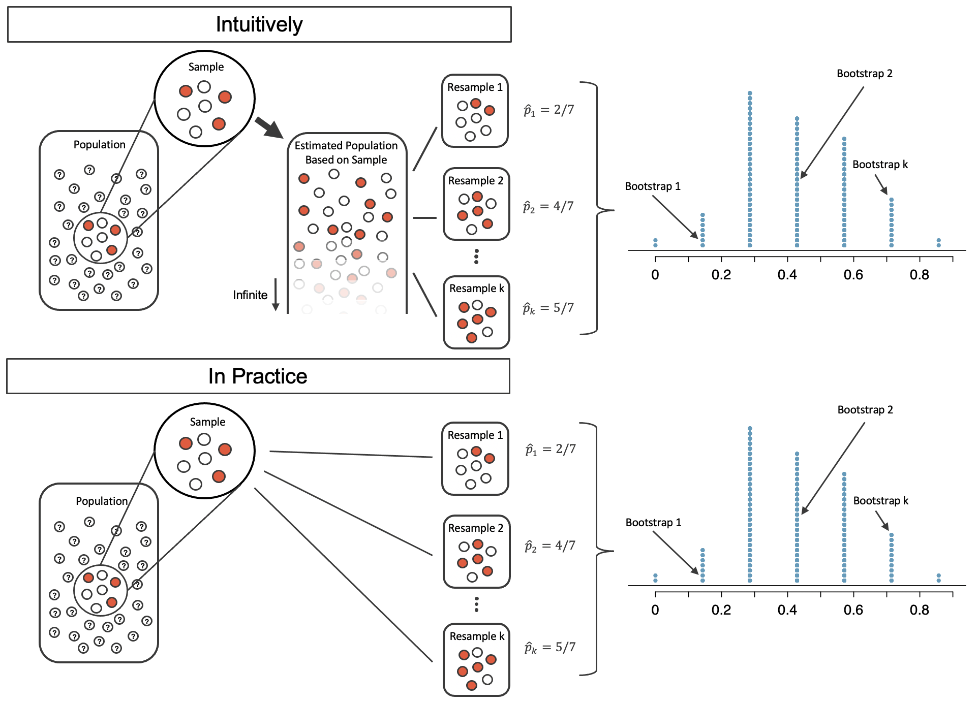
Source: IMS

Bootstrap in `R`

sample_observed <- tibble(support = c(rep(1, 900), rep(0, 600)))

set.seed(0)
slice_sample(sample_observed, n = 5) # 5 random rows from the data frame

# A tibble: 5 x 1
  support
    <dbl>
1       0
2       0
3       1
4       1
5       0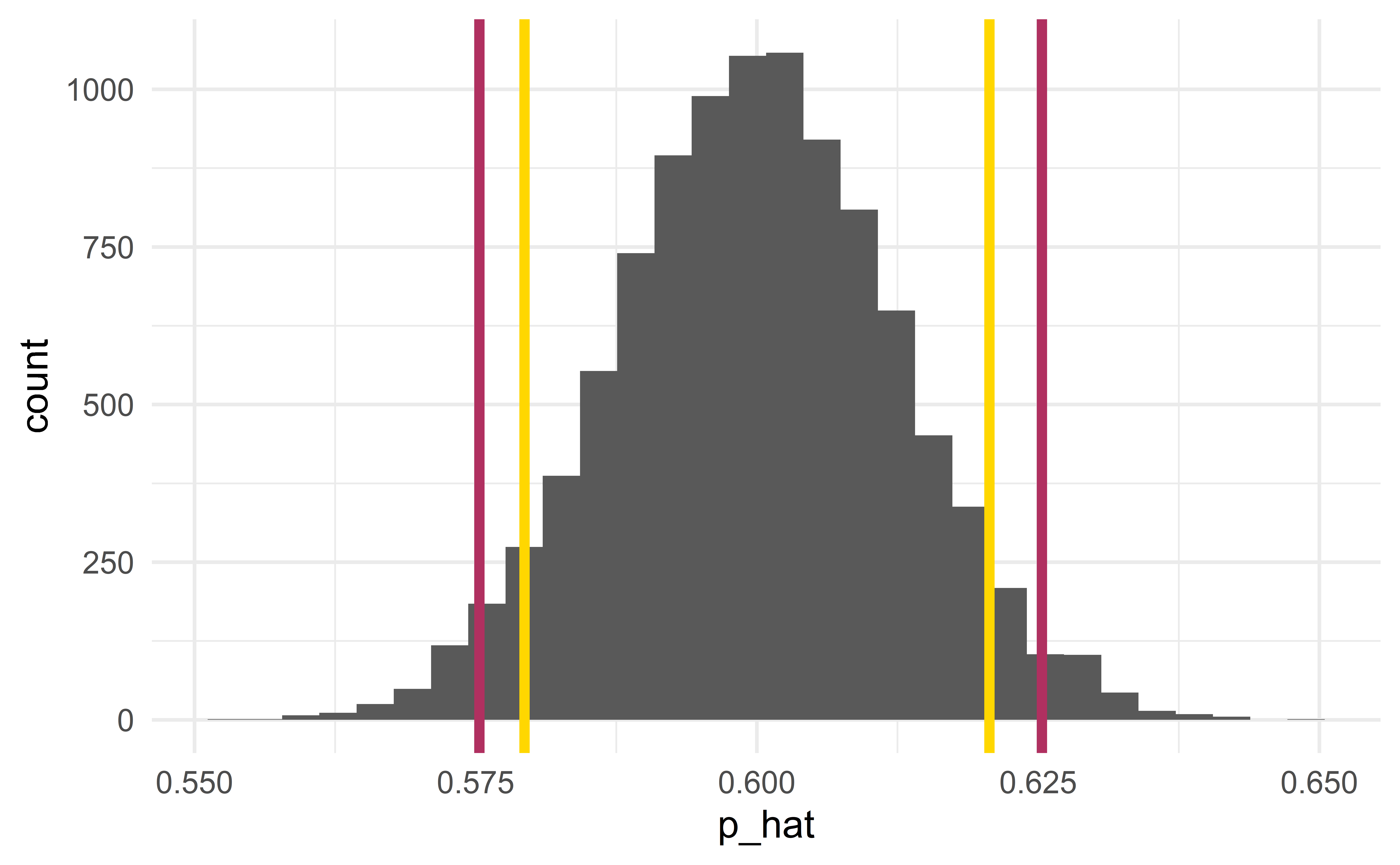

sample_bootstrap <- function(data){
  n                <- nrow(data)
  sample_bootstrap <- slice_sample(data, n = n, replace = TRUE)
  return(sample_bootstrap)
}

results <- tibble(p_hat = numeric()) # empty data frame to collect the results
set.seed(0)
for(i in 1 : 1e4){
  d_boot    <- sample_bootstrap(sample_observed) # bootstrap sample
  stat_boot <- mean(d_boot$support)              # bootstrap statistic
  results   <- results %>% add_row(p_hat = stat_boot) 
}

quantile(results$p_hat, c(0.05 , 0.95 )) # 90% CI

       5%       95% 
0.5793333 0.6206667

quantile(results$p_hat, c(0.025, 0.975)) # 95% CI (wider)

     2.5%     97.5% 
0.5753333 0.6253333

ggplot(results) + 
  geom_histogram(aes(p_hat)) + 
  geom_vline(xintercept = quantile(results$p_hat, c(0.05 , 0.95 )), col = "gold1", size = 2) + # 90% CI 
  geom_vline(xintercept = quantile(results$p_hat, c(0.025, 0.975)), col = "maroon", size = 2) # 95% CI

Group exercise - Bootstrap CI

Exercises 12.1 and 12.7

03:30

Two proportions

Setup

A population divided in two groups.

Population parameter: difference in proportion

\[ p_{diff}=p_1-p_2 \]

Sample statistics: difference in proportion in the sample

\[ \hat{p}_{diff}=\hat{p}_1-\hat{p}_2 \]

\(H_0:p_{diff}=0\) (no difference between the two groups)

\(H_a:p_{diff}\neq0\)

Example – sex discrimination

Are individuals who identify as female discriminated against in promotion decisions?

Summary results for the sex discrimination study.
	decision
sex	promoted	not promoted	Total
male	21	3	24
female	14	10	24
Total	35	13	48

Group exercise - two proportions

What are \(\hat{p}_f\), \(\hat{p}_m\) and \(\hat{p}_{diff}\)? Do you intuitively feel that the data provide convincing evidence of sex discrimination?

02:00

Hypothesis test via simulation

\(H_0:p_{diff}=0\)

\(H_a:p_{diff}\neq 0\)

Simulate many samples under \(H_0\) (no discrimination)
Determine if the observed data could have plausibly arisen under \(H_0\)

Simulating under \(H_0\)

Under \(H_0\), there is no discrimination

\(\Rightarrow\) whether someone receives a promotion is independent of their sexual identification,

\(\Rightarrow\) randomly re-assign the \(35\) promotions independently of the sexual identification.

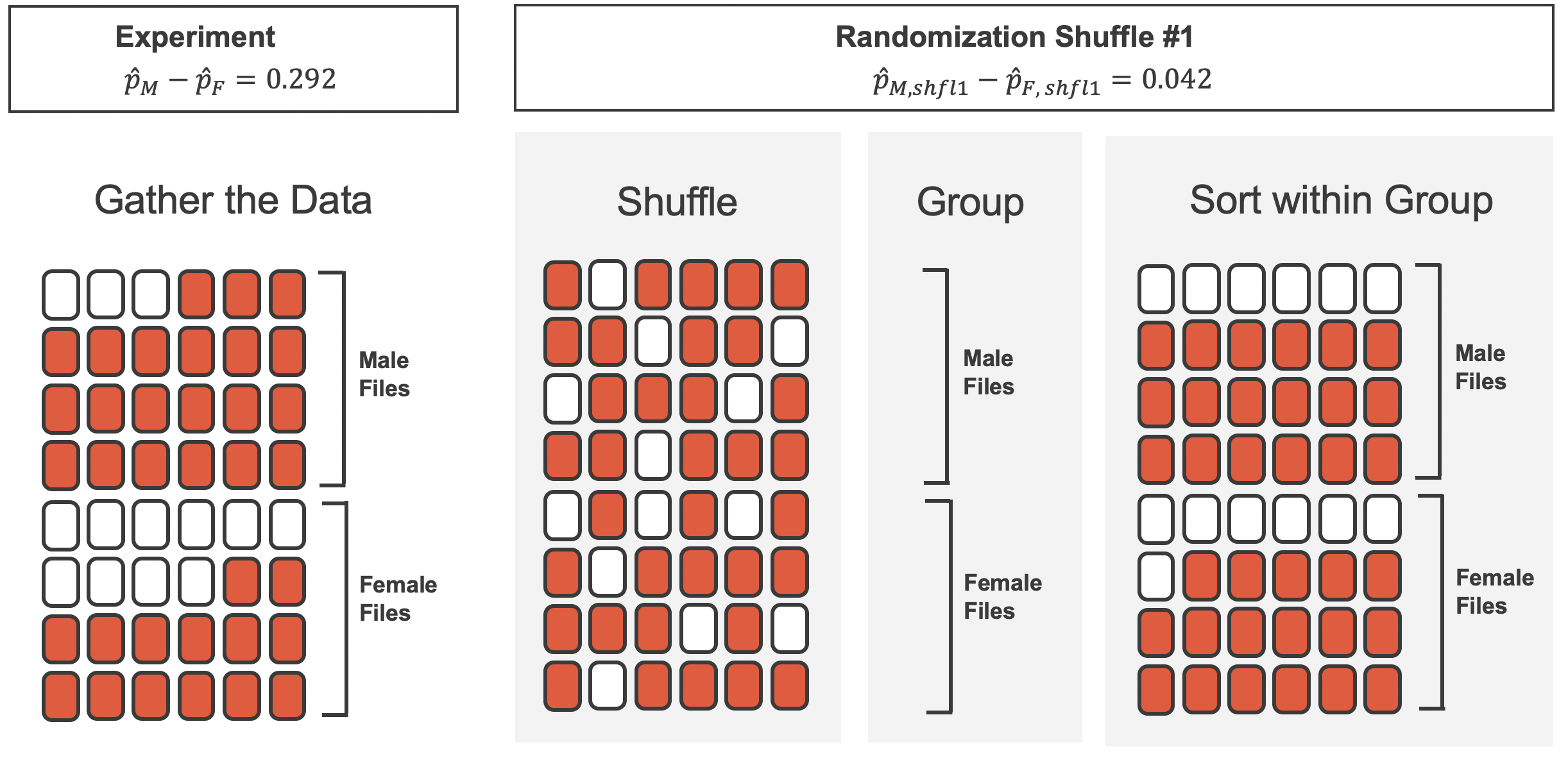Source: IMS

Simulation result

	decision
sex	promoted	not promoted	Total
male	18	6	24
female	17	7	24
Total	35	13	48

Source: IMS

d <- gender_discrimination
d_sim <- d %>% mutate(decision = sample(decision)) # shuffle the promotions
d_sim

# A tibble: 48 x 2
   gender decision    
   <fct>  <fct>       
 1 male   not promoted
 2 male   not promoted
 3 male   promoted    
 4 male   promoted    
 5 male   promoted    
 6 male   promoted    
 7 male   promoted    
 8 male   not promoted
 9 male   promoted    
10 male   not promoted
# ... with 38 more rows

Function for computing the test statistic

compute_p_diff <- function(data){
  p_hat <- data %>%
    group_by(gender) %>%
    summarize(p_hat = mean(decision == "promoted"))
  p_diff_hat <- p_hat$p_hat[1] - p_hat$p_hat[2]
  return(p_diff_hat)
}
compute_p_diff(d_sim)

[1] -0.04166667

For-loop for simulating under \(H_0\)

# Setup
results    <- tibble(p_diff_hat = numeric())
d          <- gender_discrimination

# Simulations
set.seed(0)
for(i in 1 : 1e4){
  d_sim      <- d %>% mutate(decision = sample(decision)) # simulate under H0
  p_diff_hat <- compute_p_diff(d_sim) # test statistic
  results    <- results %>% add_row(p_diff_hat = p_diff_hat)
}

Sampling distribution

p_diff_obs <- 21 / 24 - 14 / 24
p_diff_obs

[1] 0.2916667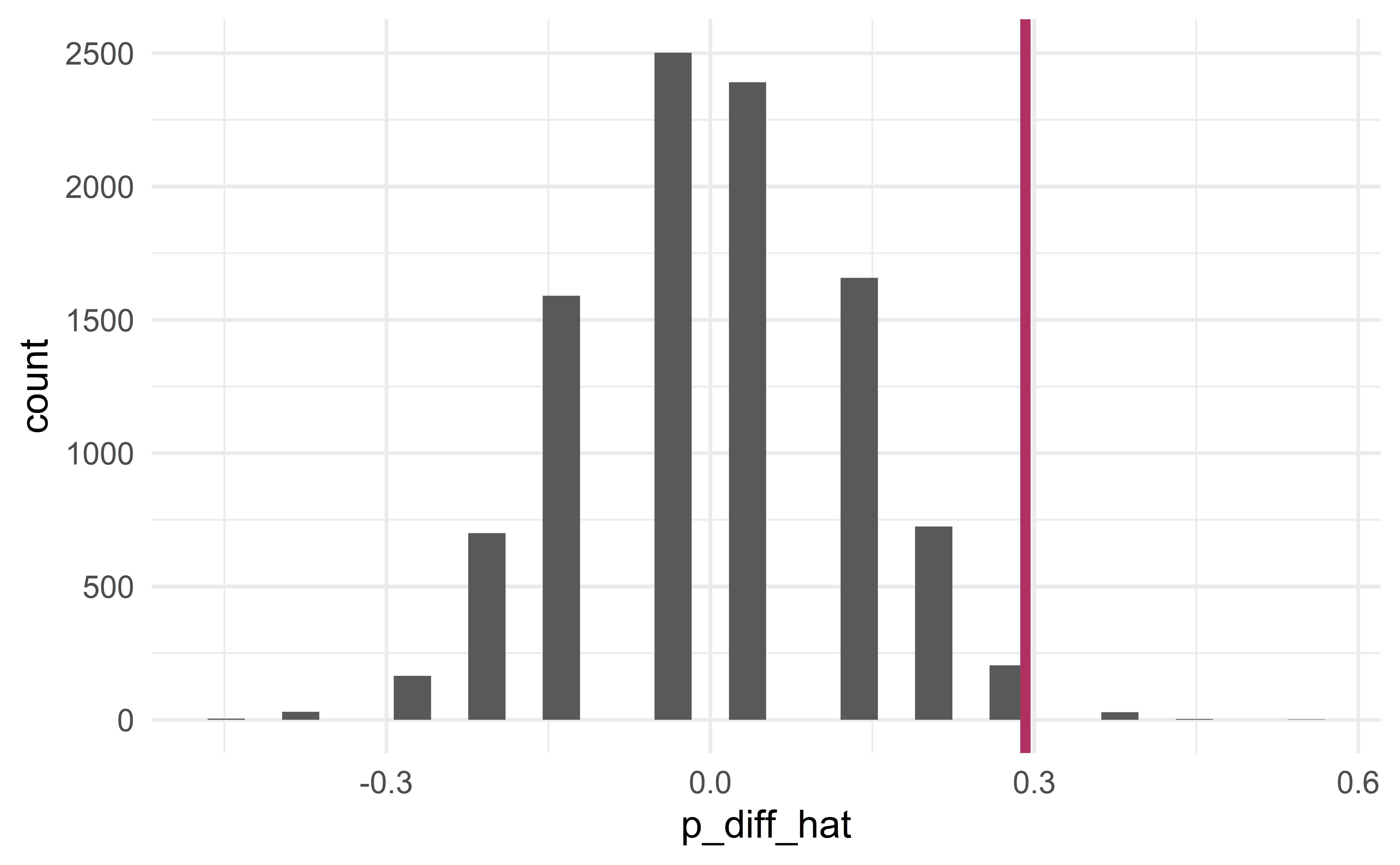

ggplot(results) + 
  geom_histogram(aes(p_diff_hat)) +
  geom_vline(xintercept = p_diff_obs, col = "maroon", size = 2)

p-value

p-value: probability that the sample statistic of a sample simulated under \(H_0\) is at least as extreme as that of the observed sample.

the probability that \(\hat{p}_{diff}^{sim}\ge\) 0.29 or \(\hat{p}_{diff}^{sim}\le\) -0.29.

results %>%
  mutate(is_more_extreme = p_diff_hat >= p_diff_obs | p_diff_hat <= -p_diff_obs) %>%
  summarize(p_value = mean(is_more_extreme))

# A tibble: 1 x 1
  p_value
    <dbl>
1  0.0435

significance level \(\alpha = 0.05\)

Using the usual significance level \(\alpha = 0.05\), we reject the null hypothesis

the observed difference in promotions is unlikely to be due to random luck
the difference is statistically significant.

Statisticians as messengers

Statisticians are just messengers; they only interpret what the data are indicating.

If you are a scientist and are not happy with the result of a statistical analysis, change the study not the statistician!

larger sample
smaller measurement errors
new variables, e.g. salary instead of promotion

Group exercise - HT

17.1 (skip part b)

03:00

Confidence interval via bootstrap

Same idea as before: sample with repetition from the observed data to construct many bootstrap samples.

Bootstrap samples \(\Rightarrow\) sampling distribution \(\Rightarrow\) CI

Bootstrap

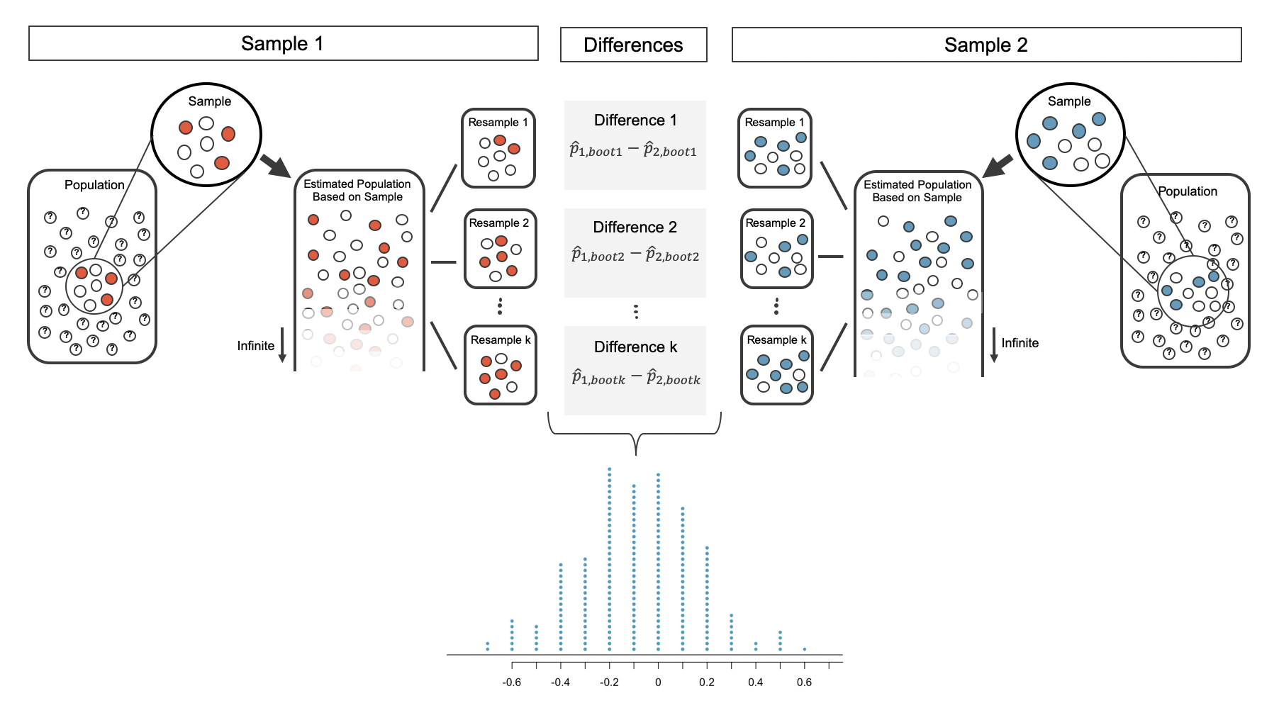
Source: IMS

Bootstrap in `R`

sample_observed_m <- gender_discrimination %>% filter(gender == "male"  )
sample_observed_f <- gender_discrimination %>% filter(gender == "female")

set.seed(0)
sample_bootstrap(sample_observed_m) # bootstrap sample

# A tibble: 24 x 2
   gender decision    
   <fct>  <fct>       
 1 male   promoted    
 2 male   promoted    
 3 male   promoted    
 4 male   promoted    
 5 male   promoted    
 6 male   not promoted
 7 male   promoted    
 8 male   promoted    
 9 male   promoted    
10 male   promoted    
# ... with 14 more rows

sample_bootstrap(sample_observed_f) # bootstrap sample

# A tibble: 24 x 2
   gender decision    
   <fct>  <fct>       
 1 female promoted    
 2 female promoted    
 3 female promoted    
 4 female promoted    
 5 female promoted    
 6 female not promoted
 7 female promoted    
 8 female not promoted
 9 female promoted    
10 female promoted    
# ... with 14 more rows

results <- tibble(p_diff_hat = numeric())
for(i in 1 : 1e4){
  d_boot_m   <- sample_bootstrap(sample_observed_m) # bootstrap sample
  d_boot_f   <- sample_bootstrap(sample_observed_f) # bootstrap sample
  p_diff_hat <- compute_p_diff(rbind(d_boot_m, d_boot_f)) # bootstrap statistic
  results    <- results %>% add_row(p_diff_hat = p_diff_hat)
}

quantile(results$p_diff_hat, c(0.05 , 0.95 )) # 90% CI

        5%        95% 
0.08333333 0.50000000

quantile(results$p_diff_hat, c(0.05 , 0.95 )) %>% signif(2) # 90% CI

   5%   95% 
0.083 0.500

quantile(results$p_diff_hat, c(0.025, 0.975)) %>% signif(2) # 95% CI

 2.5% 97.5% 
0.042 0.540

ggplot(results) +
  geom_histogram(aes(p_diff_hat))  + 
  geom_vline(xintercept = quantile(results$p_diff_hat, c(0.05 , 0.95 )), col = "gold1", size = 2) + # 90% CI 
  geom_vline(xintercept = quantile(results$p_diff_hat, c(0.025, 0.975)), col = "maroon", size = 2) # 95% CI

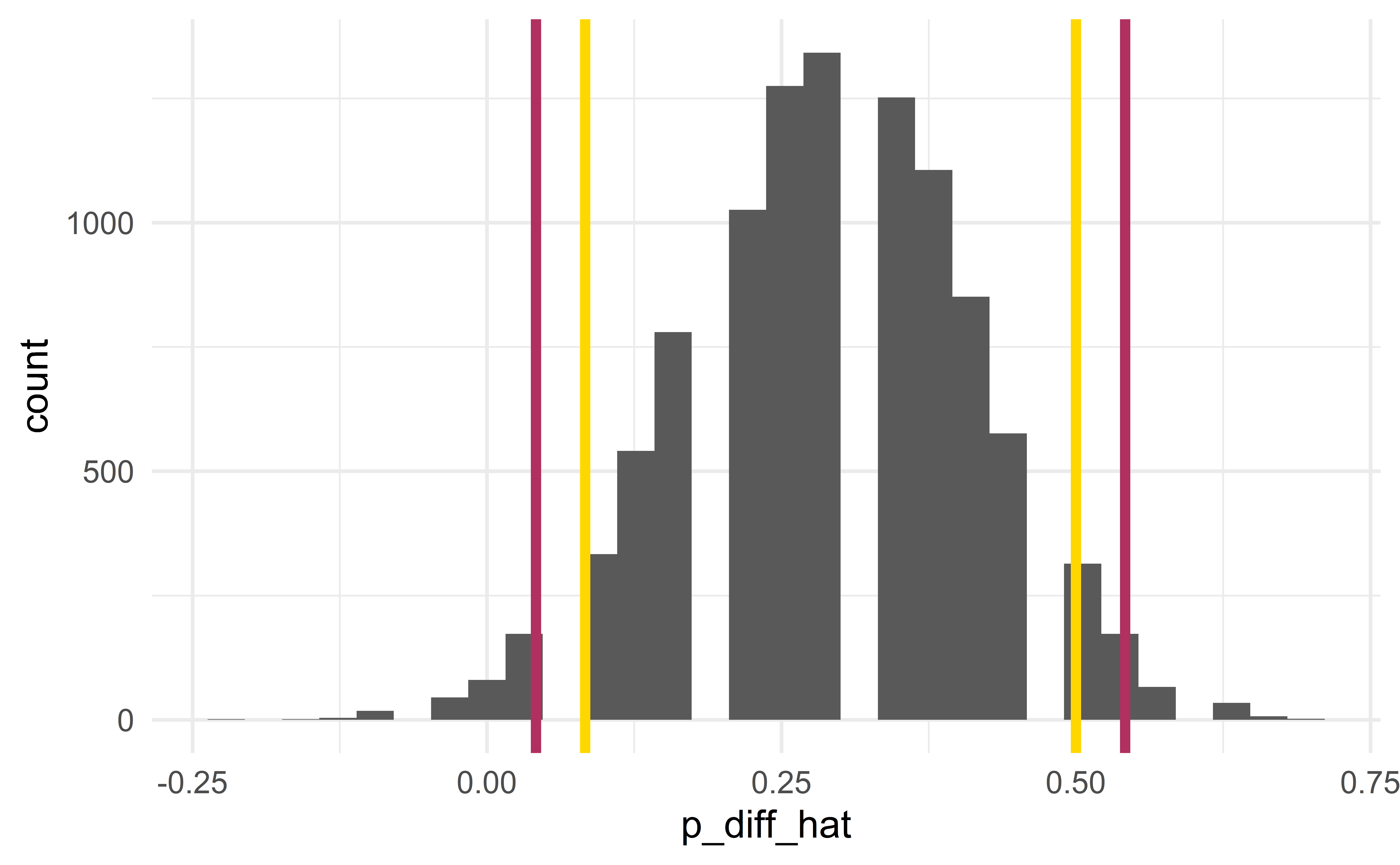
Two sides of the same coin

In the two examples, the HT and the CI agree with one another. This is not a coincidence; they will agree in the vast majority of cases!

We can show mathematically that a HT and a CI are really two sides of the same coin.

What does 90% and 95% mean?

Remember that if we could obtain multiple samples, they’d all be a bit different.

\(\Rightarrow\) the corresponding CIs would also be a bit different

A 90% CI will capture the true value of the parameter 90% of the time.
A 95% CI will be wider and thus more likely to capture the truth (95% of the time).

Trade off between being informative and true.

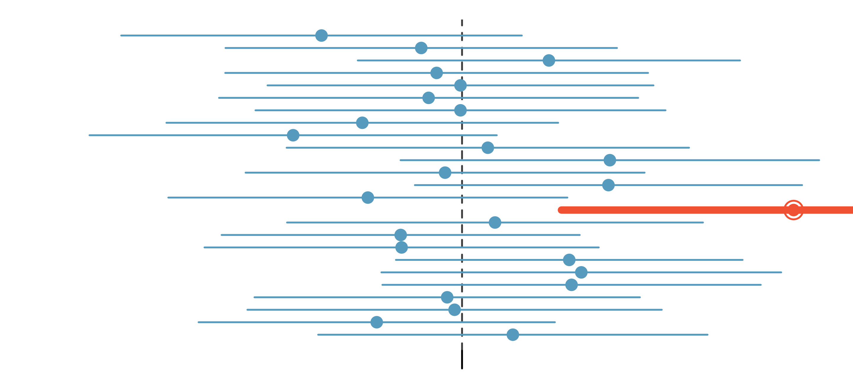
Source: IMS

Group exercises - CI

Exercises 17.3 (only do part c) and 17.5

03:00

Recap

One proportion
- HT via simulation
- CI via bootstrap
Two proportions
- HT via simulation
- CI via bootstrap

Inference for proportions

Welcome

Announcements

Recap

Outline

One proportion

Setup

Example – legalizing marijuana

Hypothesis test via simulation

Conclusion

p-value

p-value in R

p-value in practice

Confidence interval via bootstrap

Bootstrapping

Bootstrap in R

Two proportions

Setup

Example – sex discrimination

Hypothesis test via simulation

Simulating under \(H_0\)

Simulation result

Function for computing the test statistic

For-loop for simulating under \(H_0\)

Sampling distribution

p-value

significance level \(\alpha = 0.05\)

Confidence interval via bootstrap

Bootstrap

Bootstrap in R

What does 90% and 95% mean?

Recap

Recap

p-value in `R`

Bootstrap in `R`

Bootstrap in `R`