Principles of Inference

STA 101L - Summer I 2022

Raphael Morsomme

Welcome

Announcements – presentations

Presentations are < 5 minutes
QA – ask a question!
Discussion

Presentations

Announcements

Homework 5 due Sunday
Wednesday’s schedule: 3:30-4:15 lecture; 4:15-5:45 (Roy’s OH)

Recap – 1st half of course

Types of data and studies
Visualization and numerical summaries
Regression models
- linear regression
- logistic regression
- model selection

Types of data

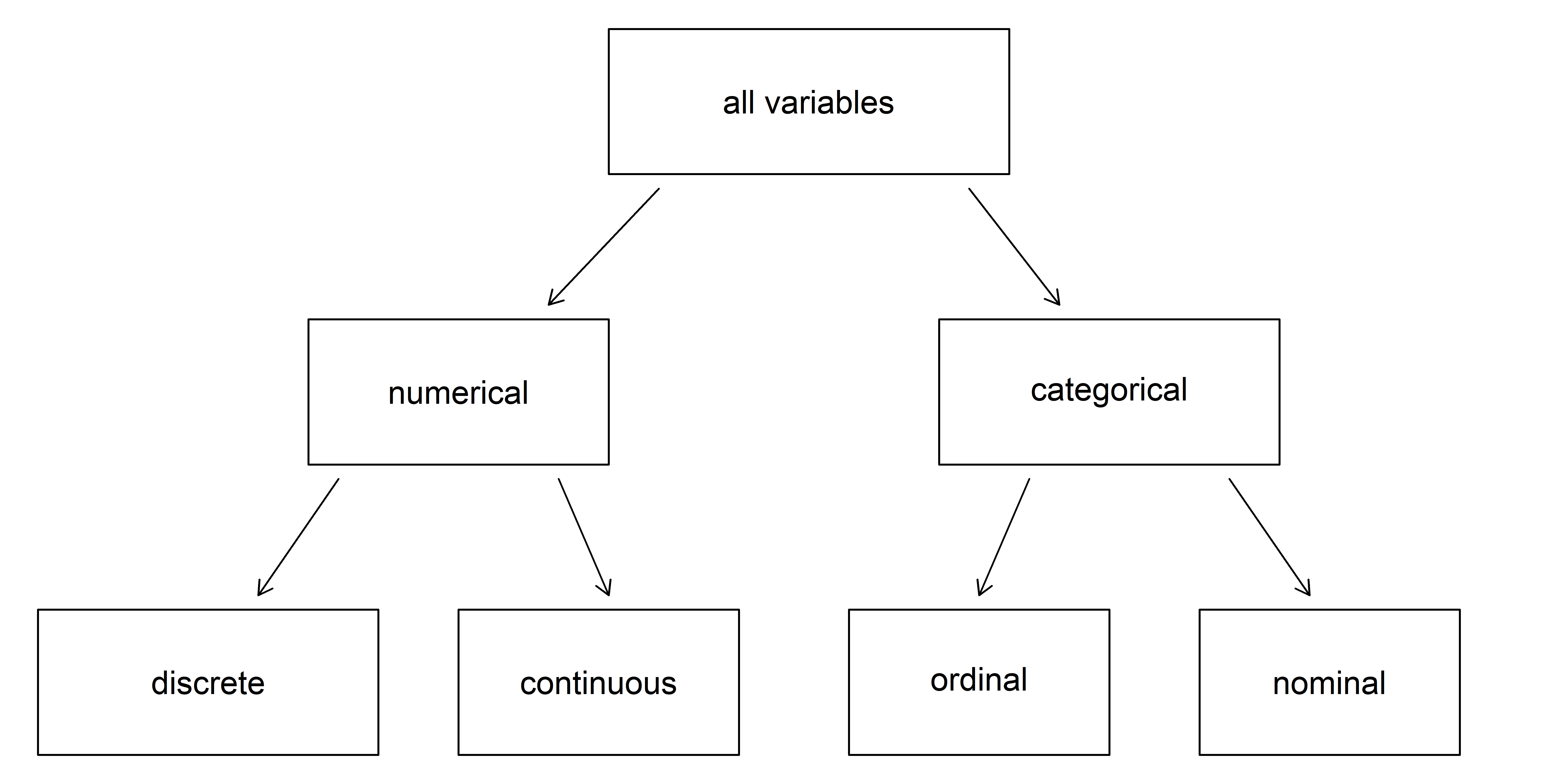
Types of variables are broken down into numerical (which can be discrete or continuous) and categorical (which can be ordinal or nominal).

Breakdown of variables into their respective types.

Source: IMS

Outline – 2nd half of course

Statistical inference
- proportions
- means
- linear and logistic regression

Outline

Statistical inference
Five cases
Hypothesis test
Confidence interval
A first glimpse of modern statistics

Statistical inference

Population parameters

We want to learn about some (unknown) parameter of some population of interest from a (small) sample of observations

Examples of parameters: proportion of vegetarian among Duke students, average weight gained by US adults during the Covid-19 pandemic, etc.

In the remainder of the course, we will always assume that we have a random sample of the population.

Group exercise - identify the parameter

Exercise 11.1

03:00

Statistical inference

Inference: estimating the population parameter from the sample.

Statistical inference: estimating the population parameter from the sample and rigorously quantify our certainty in the estimate.

Statistic

Statistic: any function of some data

e.g., average, median, iqr, maximum, variance, etc.

Sample statistic: a statistic computed on the sample

Summary statistic: a statistic used to summarize a sample

Test statistic: statistic used for statistical inference

Estimating a parameter

To estimate a population parameter, we can simply

obtain a representative sample, and
use the corresponding sample statistic as an estimate
- to estimate the median age of Duke students, simply collect a sample of students and compute their median age.

Certainty matters

A single point (the sample statistic) does not indicate how certain we are in our estimate.

If we have a large sample, we can be pretty confident that our estimates will be close to the true value of the parameter,
if we have a small sample, we know that our estimate may be far from the truth.
e.g. free throws in basketball, penalty kicks in soccer.

Statistical inference

Framework to make rigorous statements about uncertainty in our estimates

confidence intervals
- range of plausible values for the population parameter
hypothesis tests
- evaluate competing claims

Five cases

Case 1 – Single proportion

What is the proportion of vegetarians among Duke students?

Population parameter: proportion of vegetarians among Duke students $(p)$

Sample statistic: proportion of vegetarian in the sample $(\hat{p})$

Confidence interval: a range a plausible values for the population parameter $p$

for example, $(0.31, 0.43)$

Hypothesis test: is the proportion of vegetarians among Duke students $0.5$?

$H_0:p=0.5, \qquad H_a:p\neq0.5$

Case 2 – Difference between two proportions

Is the proportion of vegetarians the same among Duke undergraduate and graduate students?

Population parameter: difference between the proportion of vegetarians among Duke undergraduate and graduate students $(p_{diff} = p_{undergrad}-p_{grad})$

Sample statistic: difference in proportion of vegetarians in the sample $(\hat{p}_{diff} = \hat{p}_{undergrad} - \hat{p}_{grad})$

Confidence interval for $p_{diff}$: $(-0.05, 0.08)$

Hypothesis test: is the proportion of vegetarians the same among Duke undergraduate and graduate students?

$H_0:p_{diff}=0, \qquad H_a:p_{diff}\neq0$

Case 3 – Single mean

How much time do Duke students sleep on average per night?

Population parameter: mean amount of time that Duke students sleep per night $(\mu)$

Sample statistic: average amount of time slept in the sample $(\bar{x})$

Confidence interval for $\mu$: $(5.5, 7.5)$

Hypothesis test: Do Duke students sleep on average $8$ hours per night?

$H_0:\mu=8, H_a:\mu\neq8$

Case 4 – Difference between two means

Do Duke undergraduate and graduate students sleep on average the same amount of time per night?

Population parameter: difference between the mean amount of time that Duke undergraduate and graduate students sleep per night $(\mu_{diff} = \mu_{undergrad}-\mu_{grad})$

Sample statistic: difference between the two sample averages $(\bar{x}_{diff} = \bar{x}_{undergrad} - \bar{x}_{grad})$

Confidence interval for $\mu_{diff}$ : $(-0.5, 1)$

Hypothesis test: Do Duke undergraduate and graduate students sleep on average the same amount of time per night?

$H_0:\mu_{diff}=0, H_a:\mu_{diff}\neq0$

Case 5 – Linear regression

What is the relation between fuel consumption in the city and on the highway?

Population parameter: the coefficient $\beta_1$ is the equation $\text{hwy} \approx \beta_0 + \beta_1 \text{cty}$.

Sample statistic: the least-square estimate $\hat{\beta}_1$.

Confidence interval for $\beta_1$: $(1.05, 1.2)$

Hypothesis test: are the variables $\text{cty}$ and $\text{hwy}$ independent?

$H_0:\beta_1=0, H_a:\beta_1\neq0$

Hypothesis tests

The null hypothesis and the alternative hypothesis

Two competing hypotheses:

the null hypothesis $H_0$
- “nothing is going on”: there is no effect, no difference
the alternative hypothesis $H_a$
- “something is going on”: there is an effect, there is a difference

Example

Consider the 2nd case (difference in proportion of vegetarians between undergrad and grad students).

$H_0:$ the proportion of vegetarian is the same among undergraduate and graduate students (“nothing is going on”) $$ H_0: p_{diff}=p_{undegrad}-p_{grad}=0

\[ \]

H_a: p_{undegrad}=p_{grad} $$
$H_a:$ the proportion of vegetarians among undergraduate and graduate students is not the same (“something is going on”). $$ H_0: p_{diff}=p_{undegrad}-p_{grad}

\[ \]

H_a: p_{undegrad}p_{grad} $$

More examples

Are the Covid-19 vaccines equally effective?
- $H_0$: the vaccines are all equally effective; $H_a$: the vaccines are not all equally effective.
Does caffeine consumption affect student participation in class
- $H_0$: caffeine consumption does not affect student participation; $H_a$: caffeine consumption affects student participation.
Are men and women paid equally in the workplace?
- $H_0$: men and women are paid equally; $H_a$: men and women are not paid equally.
Have Duke students gained weight since the start of the Covid-19 pandemic?
- $H_0$: Duke student have not gained weight; $H_a$: Duke students have gained weight.

Group exercise - hypotheses

Exercises 11.3, 11.5

04:00

Natural variability

Go back to the 2nd case and suppose that $H_0$ is true.

We’ll probably still observe a small difference between undergrad and grad students in the sample.

Now suppose that $H_a$ is true.

We’ll probably observe a larger difference in the sample,
but we might also observe no difference at all,
or observe a different in the wrong direction!

Natural variability and hypothesis tests

We’ll always observe a difference

Observing a difference in the sample is not sufficient to reject $H_0$. When we collect a sample, there always is some natural variability inherent to the data.

Determining whether the observed difference is due to natural variation or provides convincing evidence of a true difference between the two groups is at the heart of hypothesis tests.

Group exercise - convincing evidence

Suppose we have a sample of Duke students with the same number of undergraduates and graduates, and $\hat{p}_{diff} = \hat{p}_{undergrad} - \hat{p}_{grad} = 0.6 - 0.4 = 0.2$. For what sample sizes $n$ do you intuitively feel that the observed difference provides convincing evidence that the two groups are different?

$n=10$ (5 undergrad and 5 grad students)
$n=20$ (10 undergrad and 10 grad students)
$n=50$ (…)
$n=100$
$n=250$
$n=500$
$n=1000$

03:00

Confidence interval

CI: range of plausible values for the population parameter.

There always is natural variability in the data.

If we draw a second sample from the population, the two samples will differ and the sample statistics will not be the same (e.g., $\hat{p}_1\neq\hat{p}_2$, $\bar{x}_1\neq\bar{x}_2$ and $\hat{\beta}^{(1)}_1\neq\hat{\beta}^{(2)}_1$).
There is thus no reason to believe that the sample statistic in the first sample is exactly equal to the population parameter (e.g. $\hat{p}_1 = p$ and $\bar{x}_1=\mu$).

Examples

What is the approval rate of the US president?
What proportion of Duke students are vegetarian?
How much weight have US adults gained since the start of the Covid-19 pandemic?

CI: range of plausible values based on a sample.

Modern statistics

Classical and modern approach

We will learn two approaches to statistical inference

classical
- pen and paper, pre-computer era
- based on simple mathematical formula
- requires the data to satisfy certain conditions
modern
- computer-intensive
- models the variability in the data by repeating a procedure many times (for-loop)
- always applicable

A first glimpse of modern statistics for HT

Individual exercise – simulation

Suppose you flip a coin 100 times and count the number of heads. In the first lecture, you were asked to identify what number of heads would make you doubt that the coin is fair.

We will run an experiment together to see if your gut feeling was correct.

Use the following commands to simulate 100 flips of a coin and count the number of heads. Repeat the experiment 5 times, keeping track of the number of heads.

set.seed(0) # change the seed for each run
flips <- rbernoulli(n = 100, p = 0.5) # 100 flips - TRUE is heads and FALSE is tails
sum(flips) # number of heads (number of TRUEs)

[1] 48

02:00

For-loop

The following for-loop does the previous experiment efficiently!

set.seed(0)
results <- tibble(prop_heads = numeric())          # empty data frame to collect the results
for(i in 1 : 1e3){                              # repeat the experiment 1,000 times
  flips      <- rbernoulli(100, p = 0.5)        # flip 100 coins (sample)
  n_heads    <- sum(flips)                      # count the number of heads
  prop_heads <- n_heads / 100                   # proportion of heads (sample statistic)
  results    <- results %>% add_row(prop_heads) # add the sample statistic to the data frame `result`
}

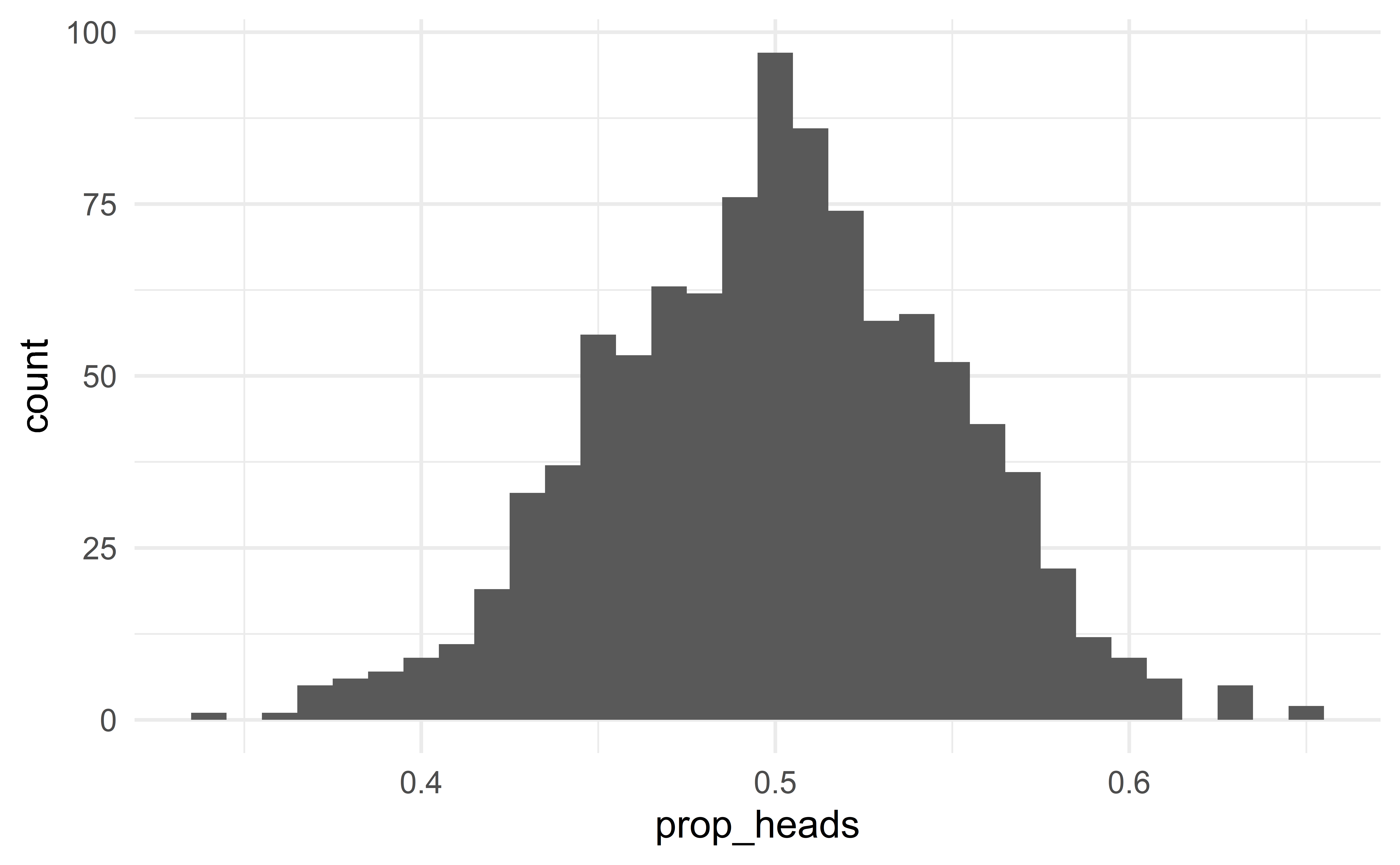
Distribution of the sample statistic $\hat{p}$ when $H_0$ is true.

ggplot(results) +
  geom_histogram(aes(prop_heads), binwidth = 0.01)

Population and parameter

Population and parameter first

Always start by defining the population and the parameter of interest.

Population: flips of the coin

Parameter: probability that a flip is head

Null and alternative hypotheses

$H_0:p=0.5$ (the coin is fair)
$H_a:p\neq0.5$ (the coin is not fair)

Like jurors in the justice system

$H_0:$ innocent (the coin is fair)
$H_a:$ guilty (the coin is not fair)

Question: do the facts (the sample) provide sufficient evidence to reject the claim that the defendant is innocent (that the coin is fair)?

If so, we reject $H_0$,
otherwise, we fail to reject $H_0$.

Never accept the null hypothesis

We never accept the null hypothesis! We only reject or fail to reject it.

ggplot(results) + 
  geom_histogram(aes(prop_heads), binwidth = 0.01) +
  geom_vline(xintercept = c(0.55, 0.65), col = "red", size = 2)

Two outcomes

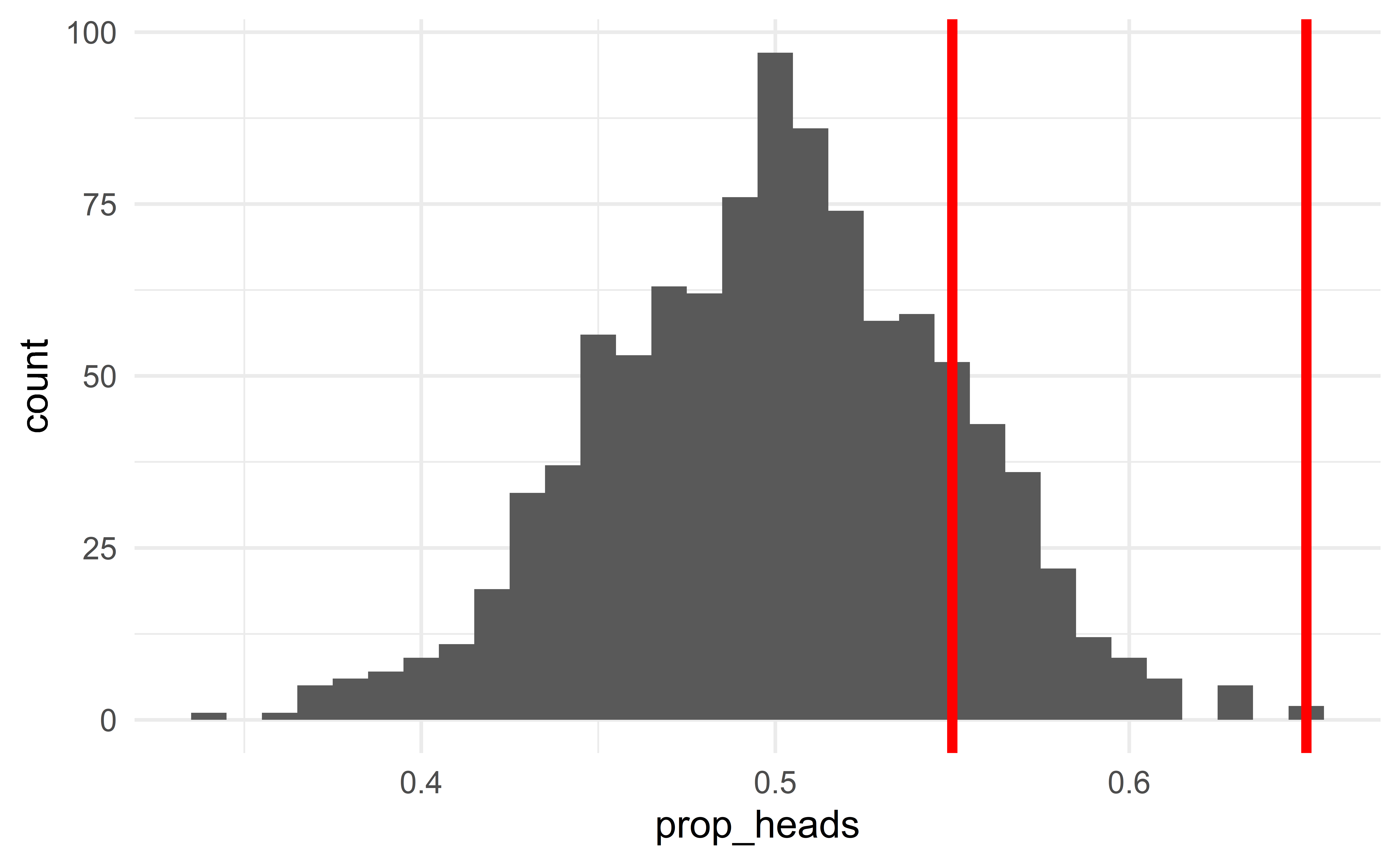
Suppose the sample consists of 55 heads of 100 flips

$\Rightarrow$ such sample is plausible under $H_0$; the observed data do not provide strong evidence against the null hypothesis; we fail to reject the claim that the coin is fair

The coin might be unfair, but the data do not provide strong evidence against fairness.

Now suppose that out of 100 flips, you observe 65 heads.

$\Rightarrow$ this result is extremely unlikely under $H_0$; the observed data provide strong evidence against the null hypothesis; we reject the claim that the coin is fair.

The coin might be fair, but a fair coin will rarely give $65$ heads out of $100$ flips.

A first glimpse of modern statistics for CI

Natural variability

Due to the natural variability of the data, each sample is different.

In practice we only get to observe a single sample. But if we could observe other samples,

they would all be a bit different

$\Rightarrow$ the sample statistics would also be different

$\Rightarrow$ the estimates would also be different.

Sample-to-sample variability

If the samples are very different

we say that the sample-to-sample variability is large.
we would not be very confident in the estimate

If the samples are all similar

we say that the sample-to-sample variability is small
we would be confident that the estimate is close to the truth

From a single sample to bootstrap samples

Problem: we only get to observe a single sample!

Solution: Use the sample to approximate the population and take repeated samples from the estimated population to simulate many samples.

Equivalent to sampling with repetition from the sample.

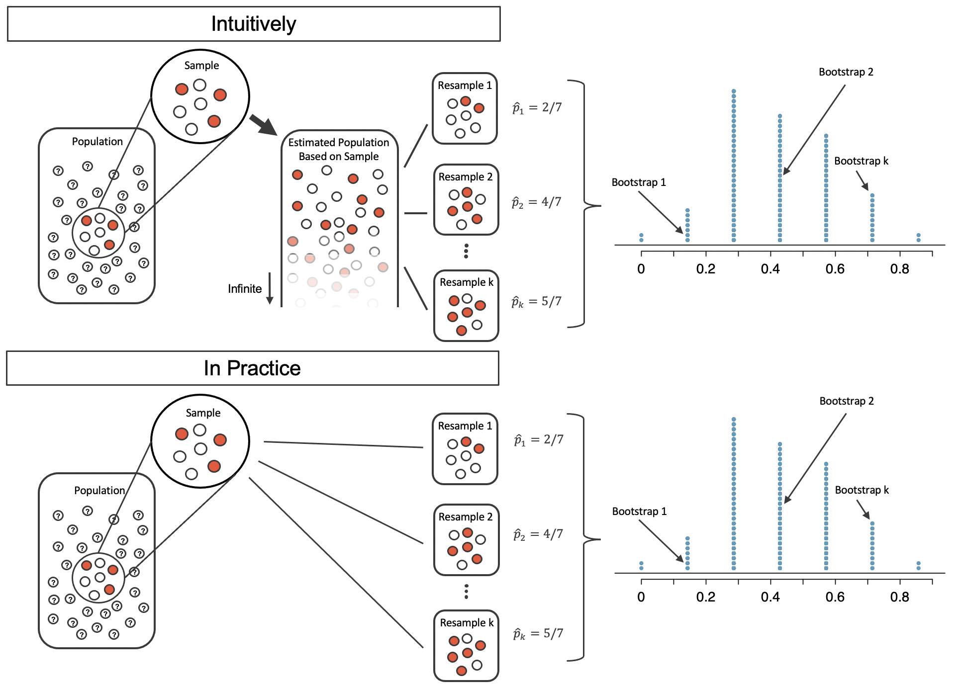
Source: IMS

From bootstrap samples to CI

Computing the sample statistic of each bootstrap sample provides its sampling distribution.

To construct a 90% CI of some parameter, we simply identify the 5th and 95th percentiles of the sampling distribution of the corresponding sample statistics.

the 5th and 95th percentiles of the sampling distribution of the median give the 90% CI for the median.

Interpretation: “We are 90% confident that the interval captures the true value of the population parameter”.

Little variability $\Rightarrow$ narrow CI

Little variability in the data

$\Rightarrow$ little sample-to-sample variability

$\Rightarrow$ little variability between bootstrap samples

$\Rightarrow$ sampling distribution of mean/proportion is concentrated

$\Rightarrow$ CI is narrow.

Much variability $\Rightarrow$ large CI

Much variability in the data

$\Rightarrow$ much sample-to-sample variability

$\Rightarrow$ much variability between bootstrap samples

$\Rightarrow$ sampling distribution of mean/proportion is diffuse

$\Rightarrow$ CI is large.

Computing bootstrap CI

d <- ggplot2::mpg
results <- tibble(mean = numeric(), sd = numeric())
for(i in 1 : 1e3){
  d_boot <- slice_sample(d, n = nrow(d), replace = TRUE) # sampling from the sample with replacement
  results <- results %>% 
    add_row(mean = mean(d_boot$cty), sd = sd(d_boot$cty)) # sample statistics of the bootstrap sample
}

ggplot(results) + 
  geom_histogram(aes(mean)) +
  geom_vline(xintercept = quantile(results$mean, c(0.05, 0.95)), col = "red", size = 2)

ggplot(results) +
  geom_histogram(aes(sd))+
  geom_vline(xintercept = quantile(results$sd, c(0.05, 0.95)), col = "red", size = 2)

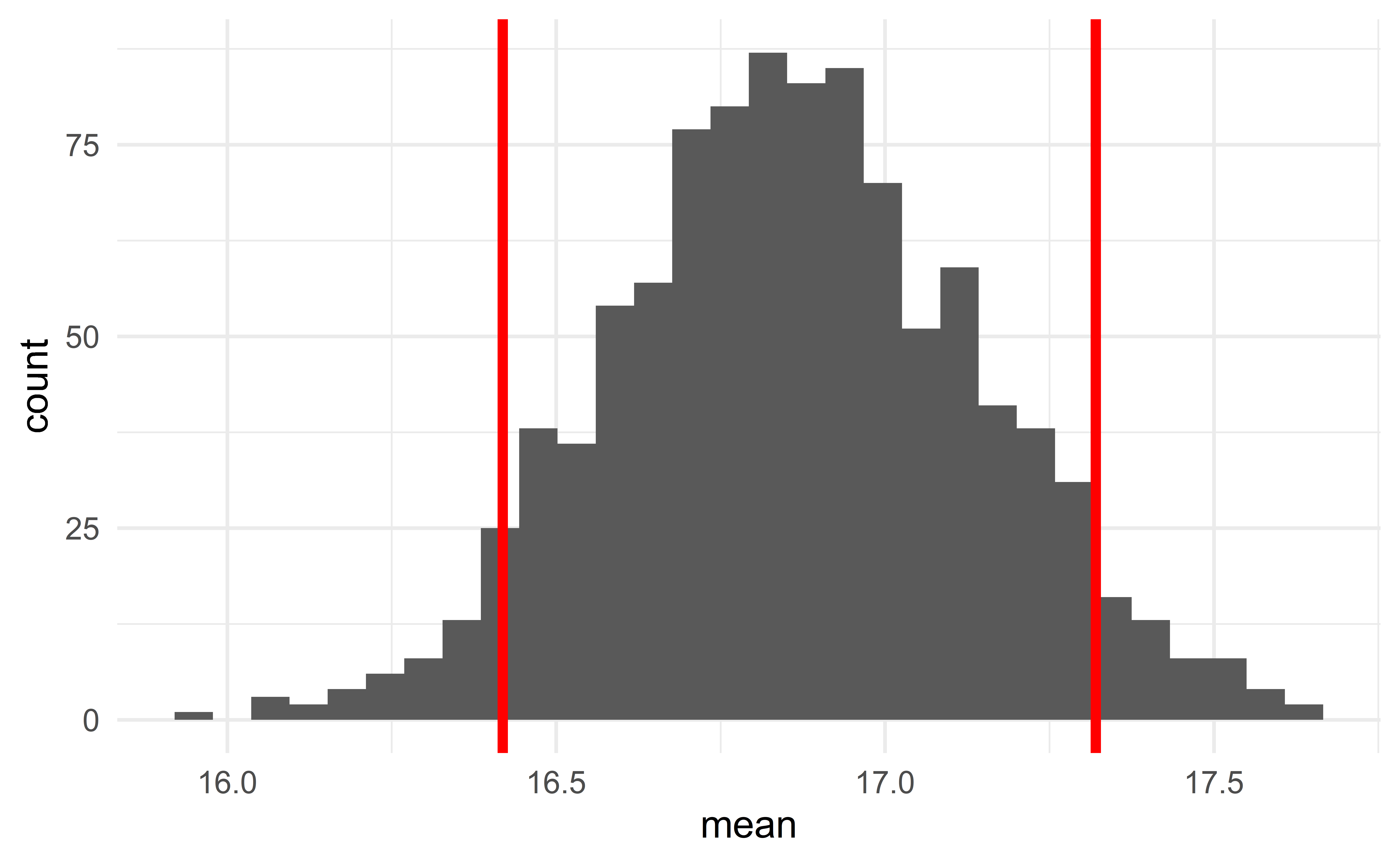
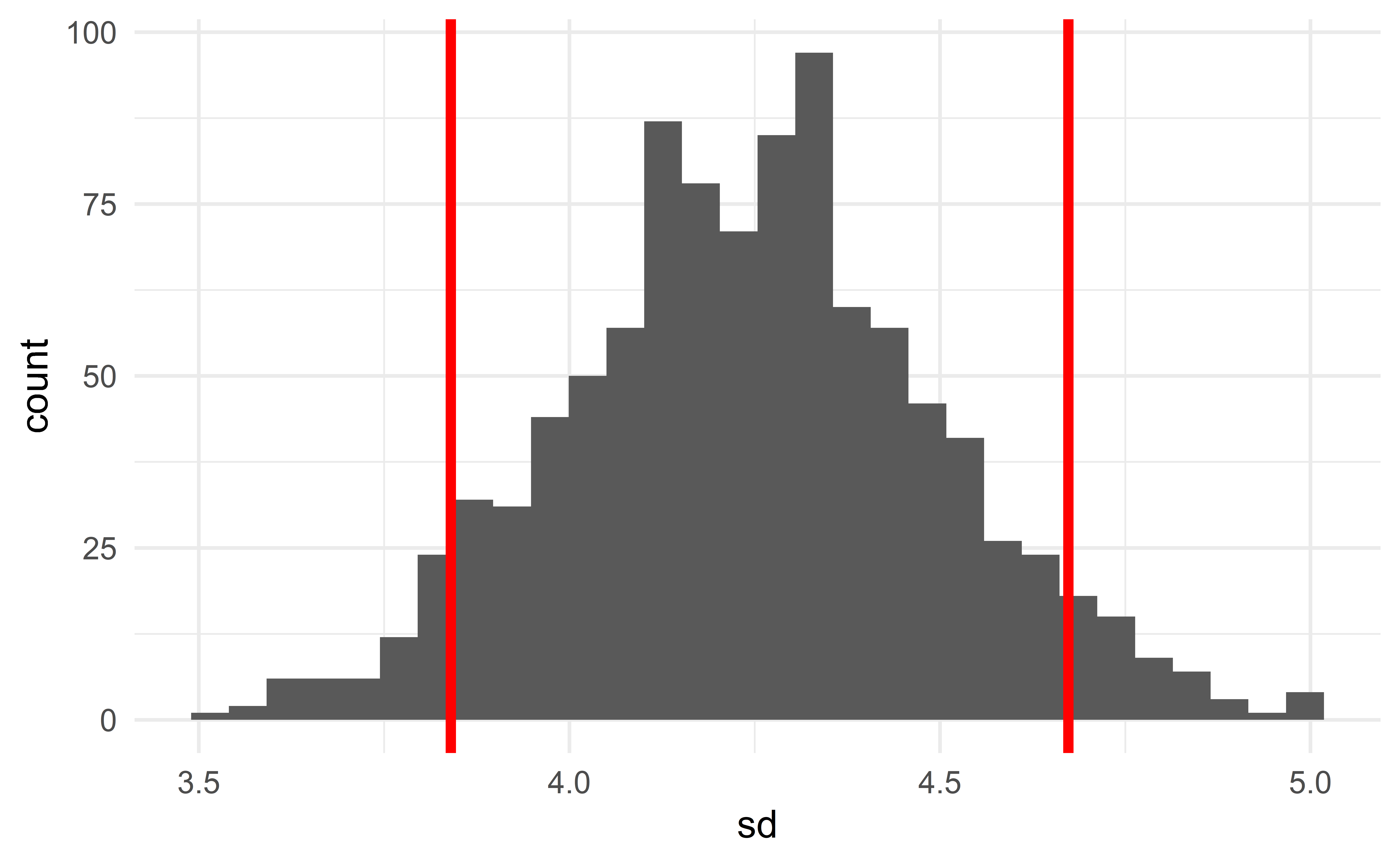
Computing the CI

# 90% bootstrap CI for the mean cty in the population
quantile(results$mean, c(0.05, 0.95))

      5%      95% 
16.41880 17.32051

# 90% bootstrap CI for the sd of cty in the population
quantile(results$sd  , c(0.05, 0.95))

      5%      95% 
3.839925 4.673212

Group exercise - bootstrap CI

Exercises 12.1, 12.3, 12.7

06:00

Group exercise - bootstrap CI

Re-use the code from the previous slide to compute a 90% bootstrap CI of the variance of cty in the population.

03:00

Recap

Statistical inference
Five cases
- single proportion
- difference between two portions
- single mean
- difference between two means
- regression parameters
Hypothesis test
Confidence interval
A first glimpse of modern statistics

Principles of Inference

Welcome

Announcements – presentations

Presentations

Announcements

Recap – 1st half of course

Types of data

Outline – 2nd half of course

Outline

Statistical inference

Population parameters

Statistical inference

Statistic

Estimating a parameter

Certainty matters

Statistical inference

Five cases

Case 1 – Single proportion

Case 2 – Difference between two proportions

Case 3 – Single mean

Case 4 – Difference between two means

Case 5 – Linear regression

Hypothesis tests

The null hypothesis and the alternative hypothesis

Example

More examples

Natural variability

Natural variability and hypothesis tests

Confidence interval

Confidence interval

Examples

Modern statistics

Classical and modern approach

A first glimpse of modern statistics for HT

For-loop

Population and parameter

Null and alternative hypotheses

Like jurors in the justice system

Two outcomes

A first glimpse of modern statistics for CI

Natural variability

Sample-to-sample variability

From a single sample to bootstrap samples

From bootstrap samples to CI

Little variability \(\Rightarrow\) narrow CI

Much variability \(\Rightarrow\) large CI

Computing bootstrap CI

Computing the CI

Recap

Recap