Logistic Regression

STA 101L - Summer I 2022

Raphael Morsomme

Welcome

Announcements

Recap

  • Simple and multiple lrm

    • numerical response
  • model selection

    • overall criterion

    • predictive performance

    • stepwise procedures

Outline

  • Modeling a binary response
  • Logistic regression
  • One predictor
  • Multiple predictors

Modeling a binary response

Example – Stanford University Heart Transplant Study

  • Goals: to determine whether an experimental heart transplant program increases lifespan

  • observations: patients

  • response: survival after 5 years (binary)

  • predictors: age, prior surgery, waiting time for transplant.

Data

d <- heart_transplant
d
# A tibble: 103 x 8
      id acceptyear   age survived survtime prior transplant  wait
   <int>      <int> <int> <fct>       <int> <fct> <fct>      <int>
 1    15         68    53 dead            1 no    control       NA
 2    43         70    43 dead            2 no    control       NA
 3    61         71    52 dead            2 no    control       NA
 4    75         72    52 dead            2 no    control       NA
 5     6         68    54 dead            3 no    control       NA
 6    42         70    36 dead            3 no    control       NA
 7    54         71    47 dead            3 no    control       NA
 8    38         70    41 dead            5 no    treatment      5
 9    85         73    47 dead            5 no    control       NA
10     2         68    51 dead            6 no    control       NA
# ... with 93 more rows

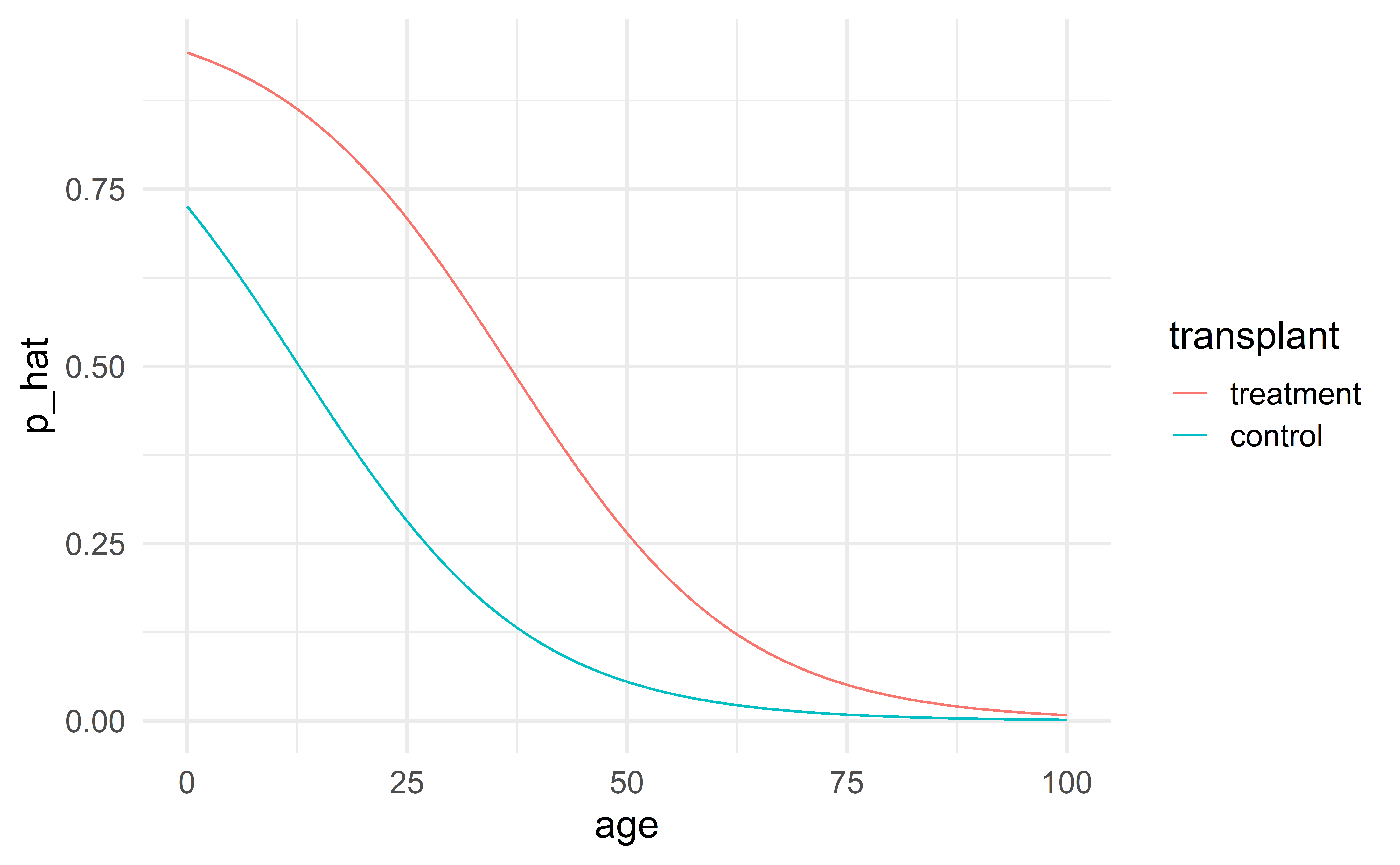
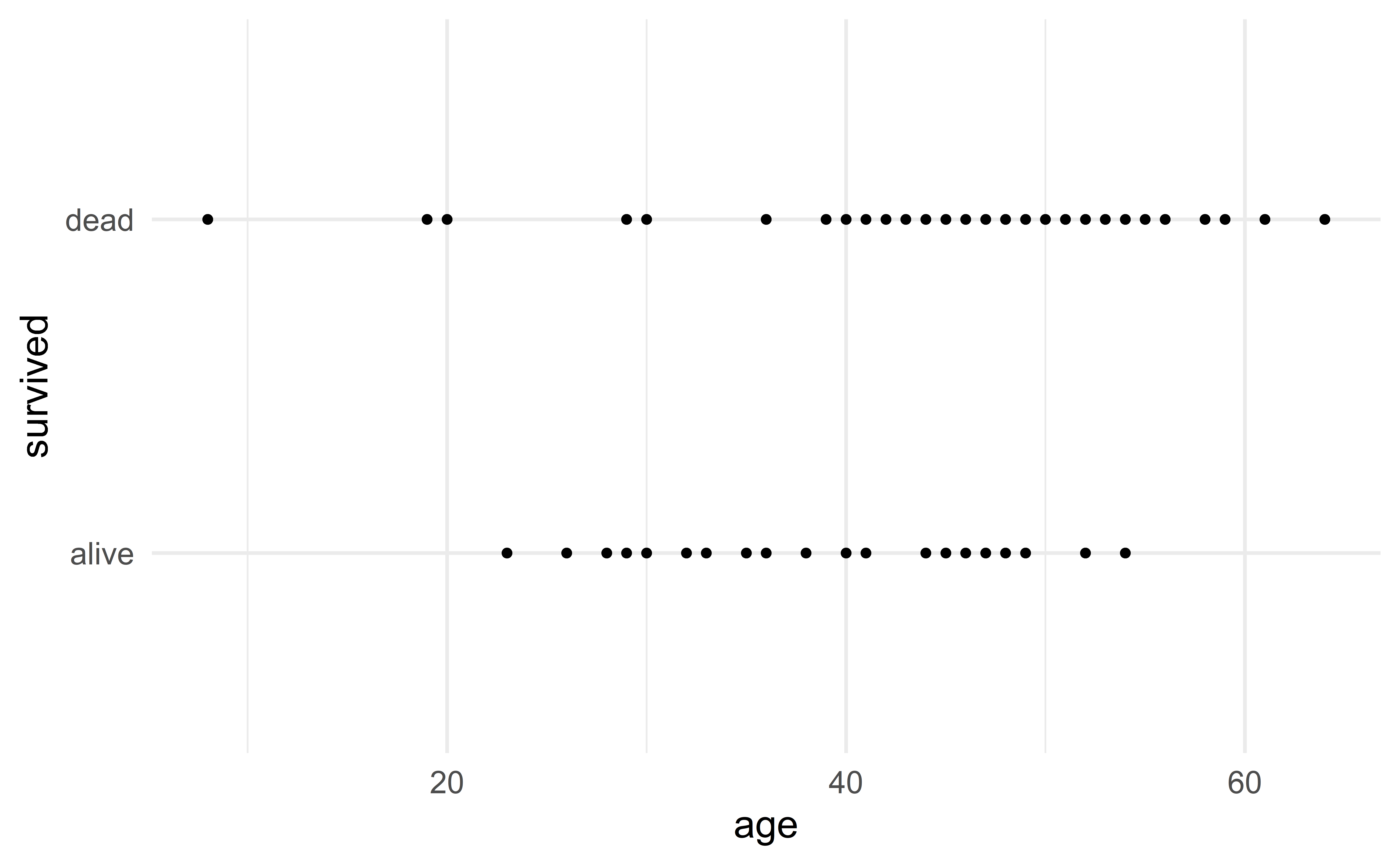
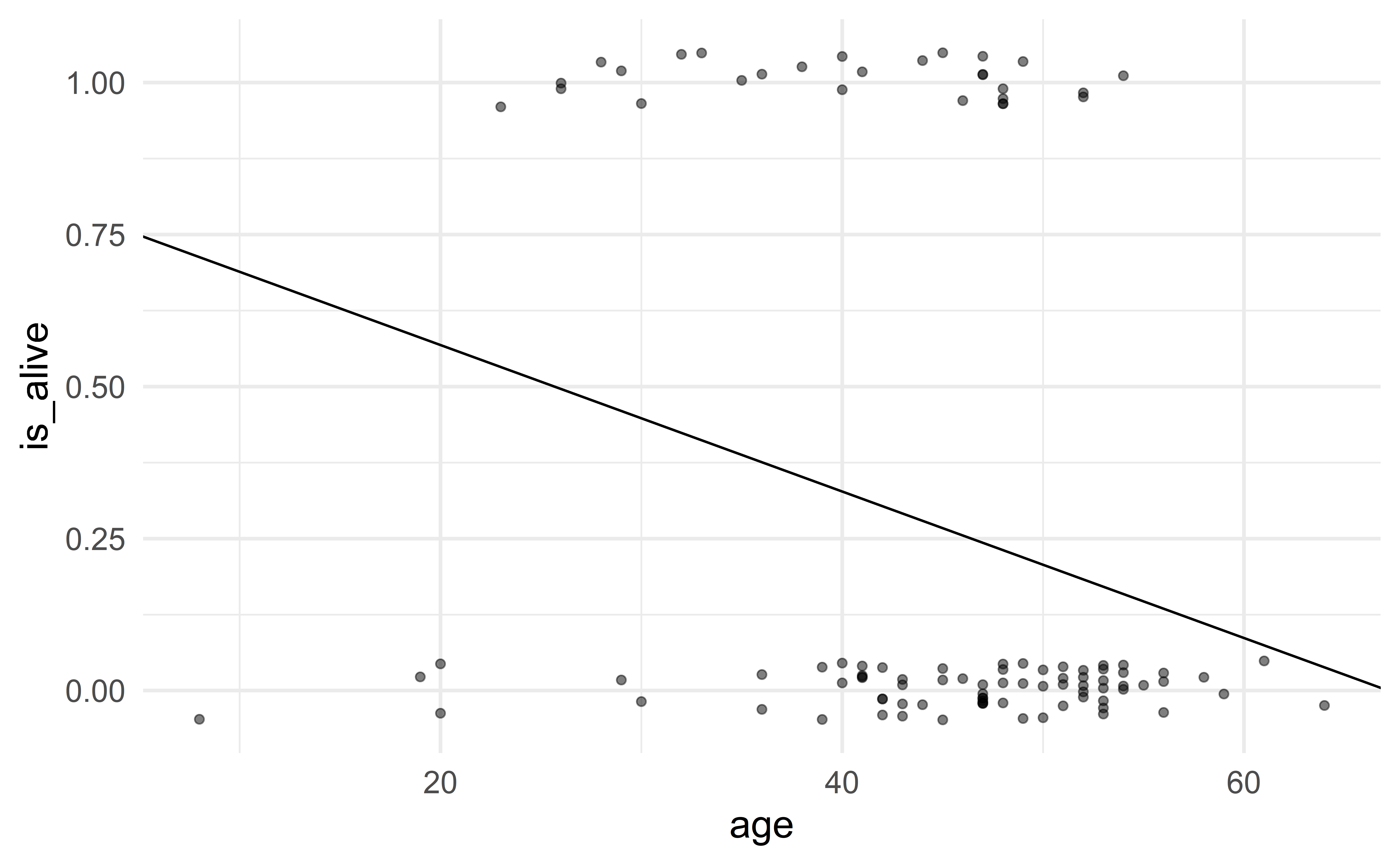
Effect of age on survival

d %>%
  ggplot(aes(x = age, y = survived)) +
  geom_point()

d %>%
  ggplot(aes(x = age, y = survived)) +
  geom_jitter(     # add random noise to point location
    width = 0,     # horizontal jitter
    height = 0.05, # vertical jitter
    alpha = 0.5    # transparency
    )

Binary response

  • Technical problem: levels of the response are labels

    • can’t fit a regression model to words, only to numbers
  • use mutate to create a binary variable (either 0 or 1)

d <- d %>%
  mutate(is_alive = if_else(survived == "alive", 1, 0))

ggplot(data = d, aes(x = age, y = is_alive)) + 
  geom_jitter(width = 0, height = 0.05, alpha = 0.5)

Linear regression?

Intuitively, age should be a good predictor of survival.

Let us fit a linear regression model

\[ \text{is_alive} \approx \beta_0 + \beta_1 age \]

m_lrm <- lm(is_alive ~ age, data = d)

ggplot(data = d, aes(x = age, y = is_alive)) + 
  geom_jitter(width = 0, height = 0.05, alpha = 0.5) +
  geom_abline(intercept = 0.80955, slope = -0.01205)

Problems with linear regression

  • The response is not continuous

    • unlike fuel consumption, tree volume or newborn weight
  • nonsensical predictions, even for reasonable value of age.

Group exercise - limitation of linear regression

What is the prediction for a 70-year-old patient?

02:00

Generalized linear models

GLMs

Generalized linear models (GLMs – STA310) extend the linear regression framework to settings where the response variable is restricted:

  • logistic regression with binary response

  • multinomial regression with nominal (categorical) response, e.g. voting in multiparty systems

  • ordinal regression with ordinal (categorical) response, e.g. course letter grade

  • poisson regression with count response, e.g. number of children

  • gamma regression with positive response variable, e.g. mpg, insurance costs

  • beta regression with continuous response between 0 and 1 (percentage), e.g. cancer rates in counties

Logistic regression

Logistic regression

  • Example of a generalized linear model

  • We’ll focus on implementation and interpretation

  • Useful for inference project (not the prediction project)

Logistic regression: model the probability of success \(p\) based on a set of predictors \(X_1, \dots, X_p\).

Binary outcome and probability

Let \(Y_i\) denote the response of person \(i\).

The logistic regression model assumes that

\[ Y_i = \begin{cases} 1 \text{ (success)}, \text{with probability } p_i, \\ 0 \text{ (failure)}, \text{with probability } 1-p_i. \end{cases} \]

where \(p_i\) denotes the probability of success (survival) of person \(i\).

Modeling a probability with linear regression?

We saw that we cannot model \(p\) with a lrm (\(p \approx \beta_0 + \beta_1\text{age}\))

  • \(0\le p_i\le1\)

  • …but \(\beta_0 + \beta_1 \text{age}\) may be negative or larger than 1!

    • in fact, the regression line extends infinitely in either either direction

Warning

Binary variables should not be modeled using linear regression!

Modeling a probability with logistic regression

Intuitively, an older patient should have a smaller probability of surviving.

\(\Rightarrow\) We want a model that associates a smaller probability \(p\) for a patient with a larger year variable.

\(\Rightarrow\) We need to find a way to go from age (could be any number) to \(p\) (between 0 and 1)

The logit transformation

Consider the logit transformation

\[ p = \dfrac{e^{\mu}}{1+e^{\mu}} \]

where \(\mu\) can be any number.

tibble(mu = seq(-7.5, 7.5, by = 0.01)) %>%
  mutate(p = exp(mu)/(1+exp(mu))) %>%
  ggplot() + 
  geom_line(aes(x = mu, y = p))

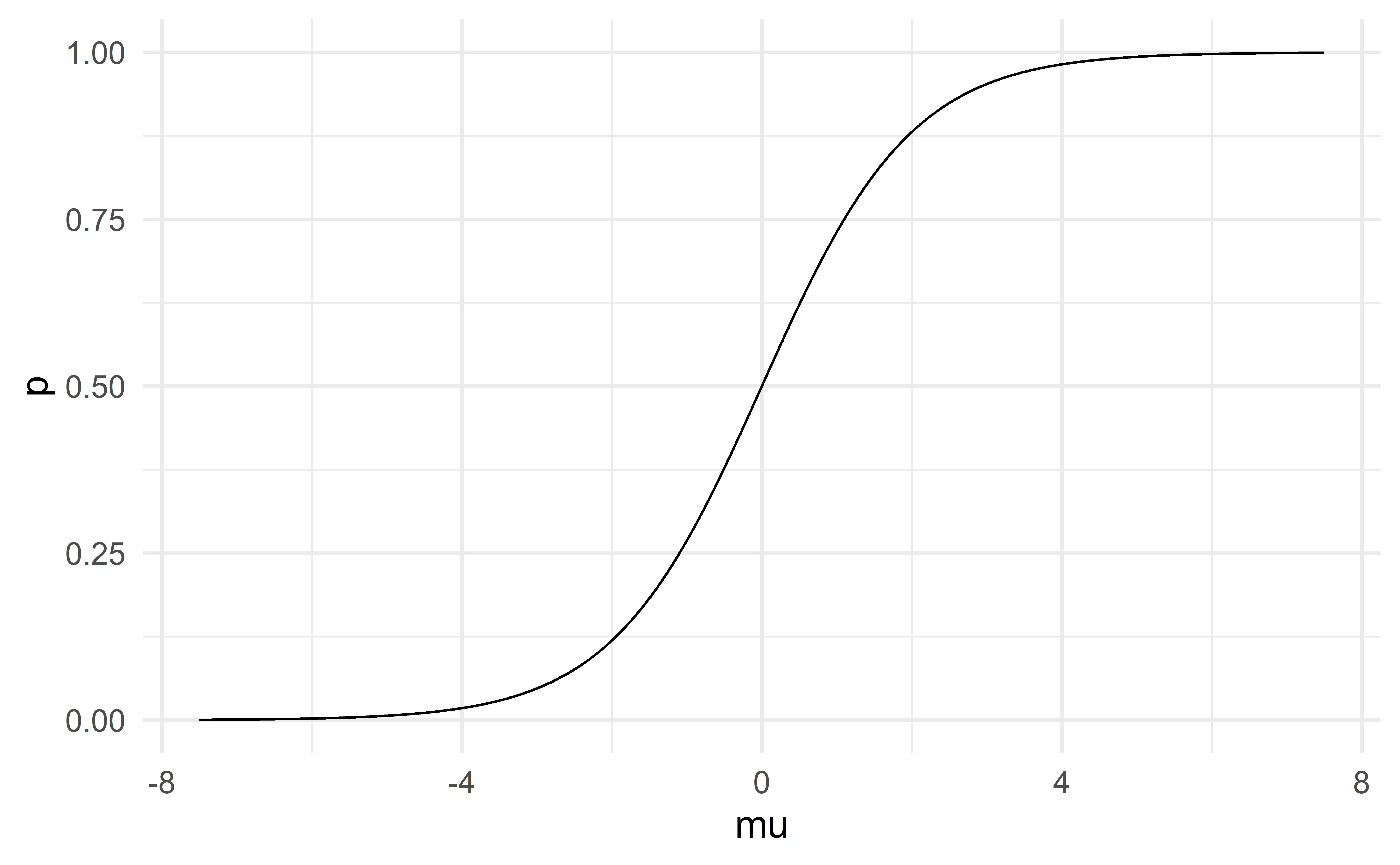
Note that \(\dfrac{e^{\mu}}{1+e^{\mu}}\) is bounded between 0 and 1.

Moreover, larger values of \(\mu\) will give larger \(p\), and smaller \(\mu\) will give smaller \(p\).
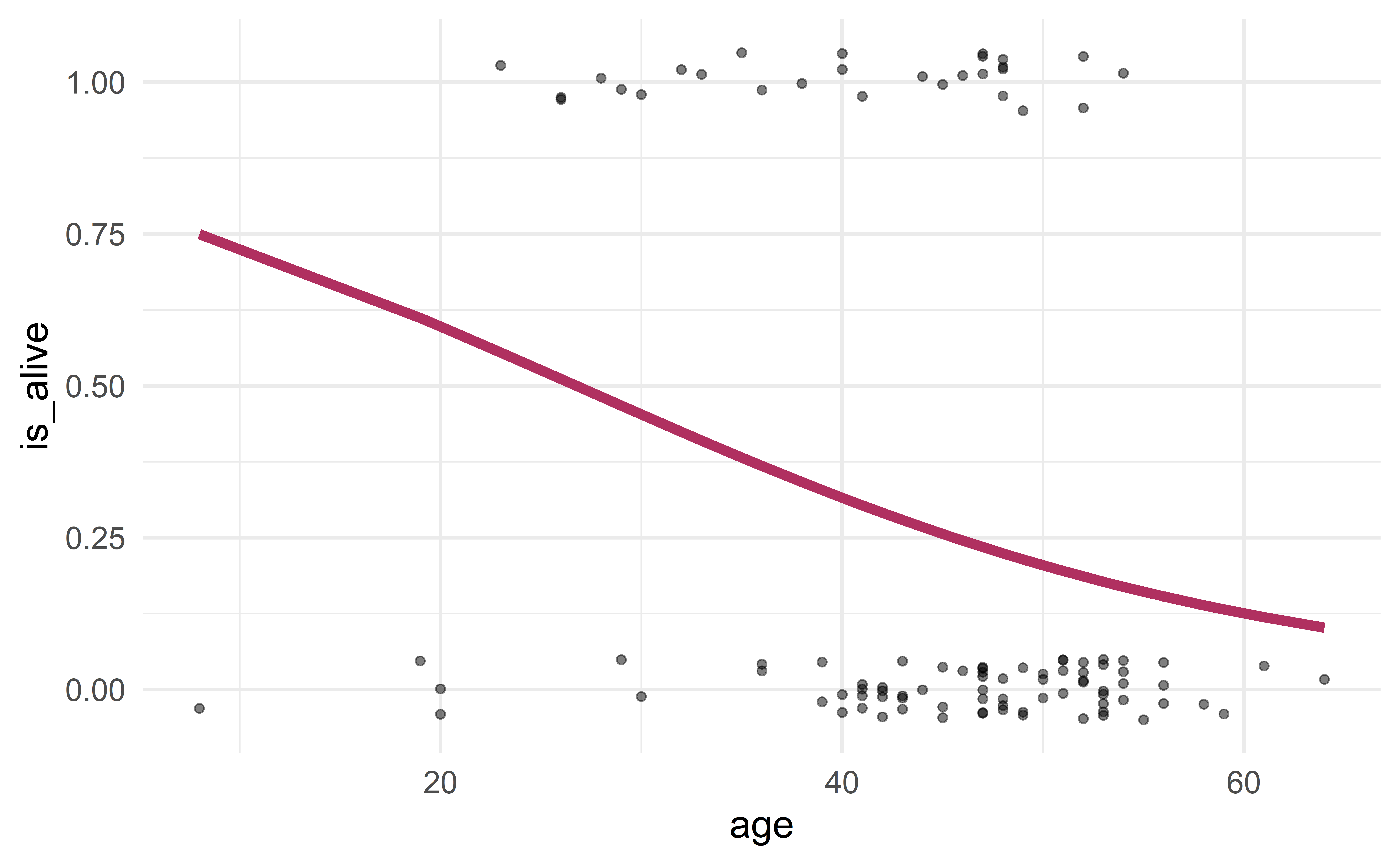
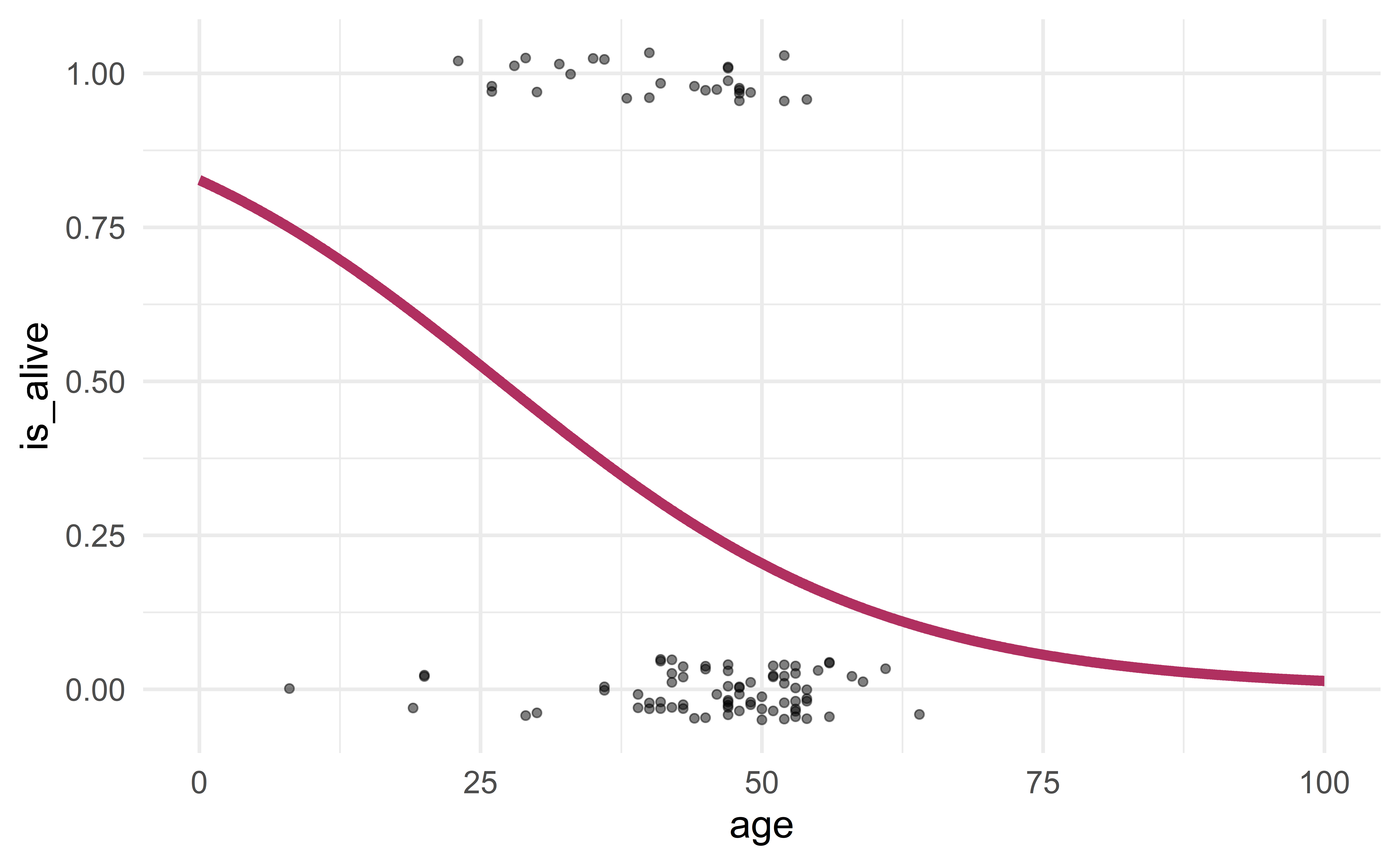
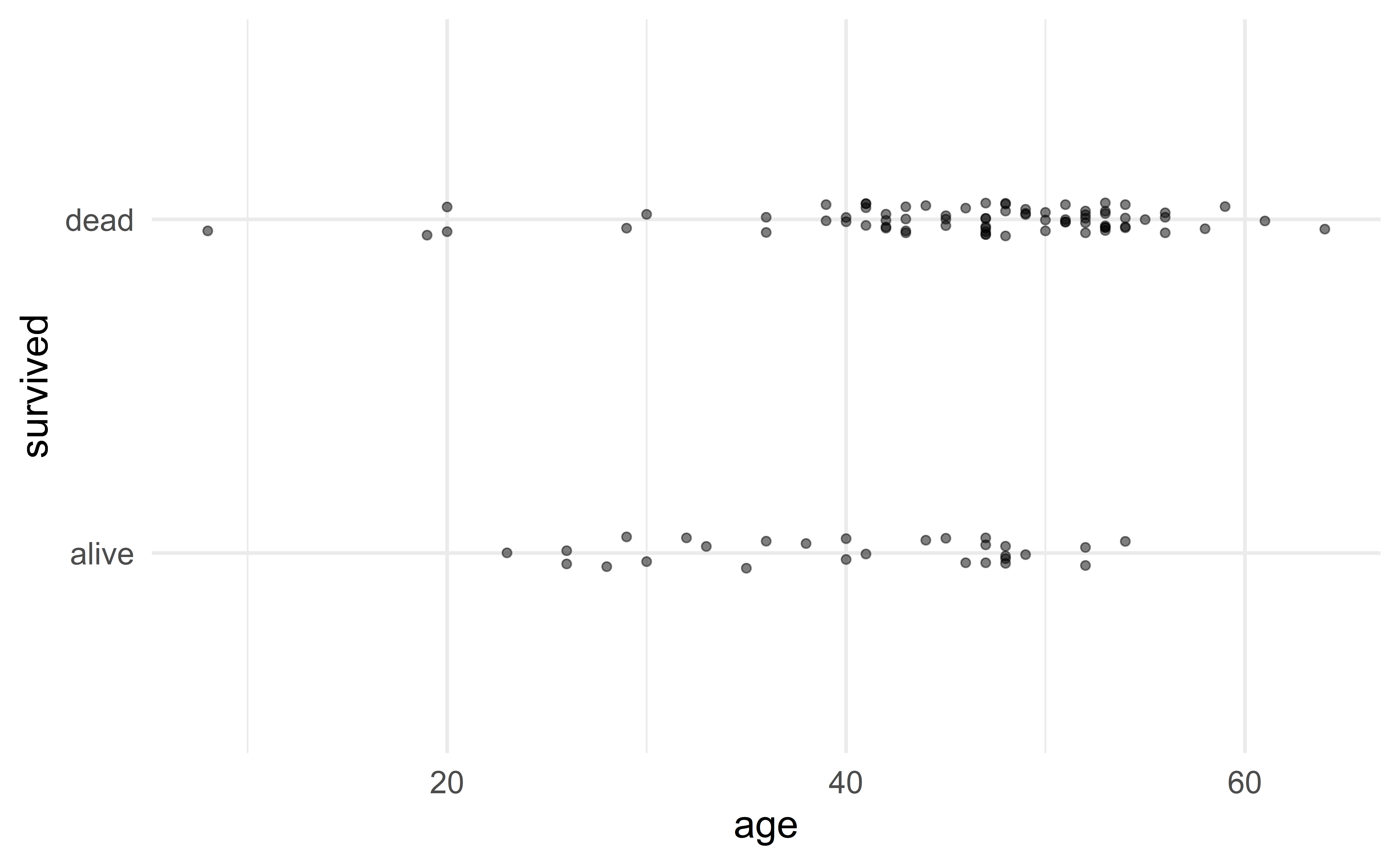
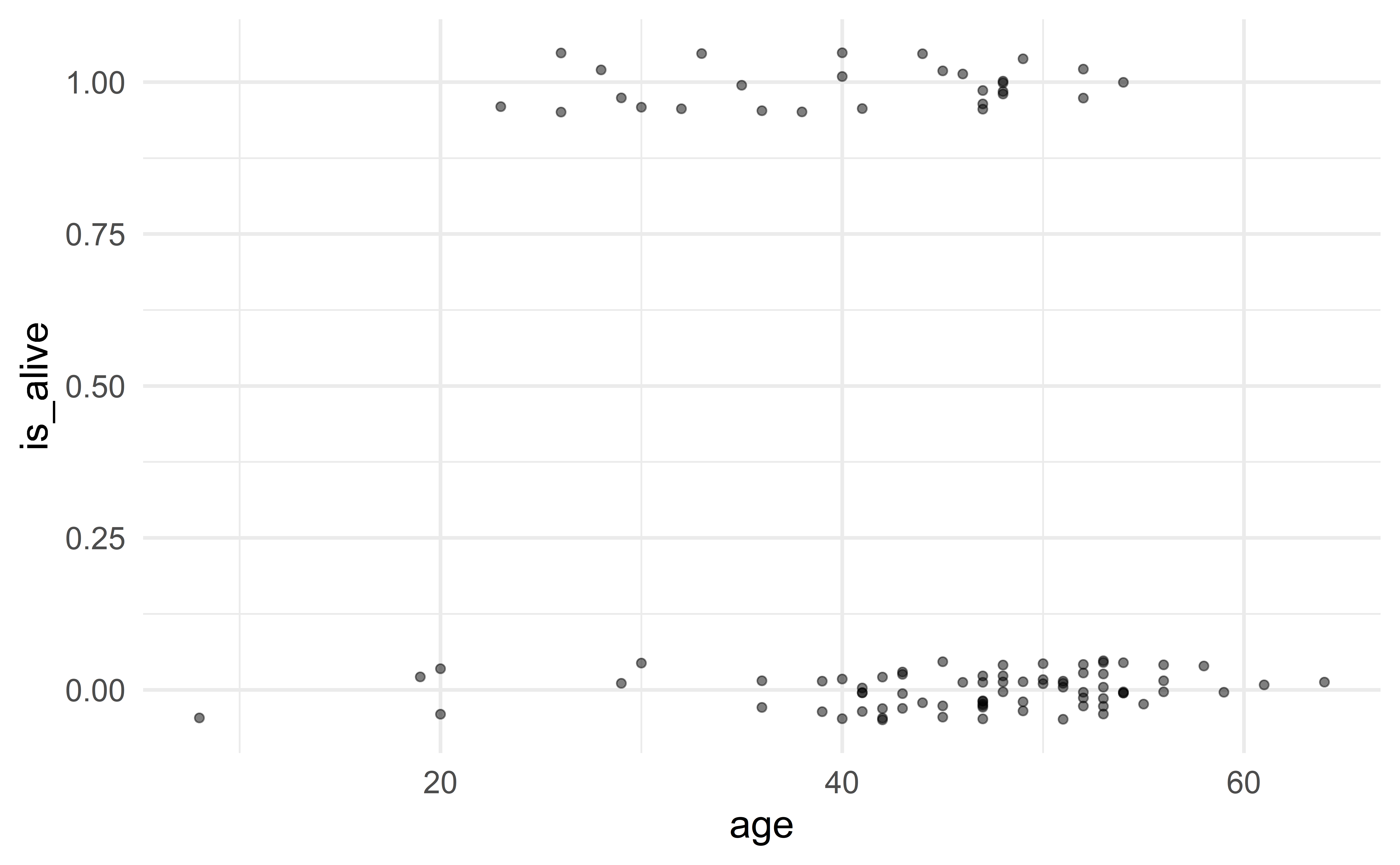
Group exercise - logit transformation

  • What value of \(p\) corresponds to

    • \(\mu = 0.5\)?

    • \(\mu = 2\)?

    • \(\mu = -2\)?

  • What value of \(\mu\) gives

    • \(p=0.5\)?

    • \(p=0.9\)?

    • \(p=0.1\)?

03:00

Modeling \(\mu\)

We can now simply model \(\mu\) using a simple lrm with age

\[ \mu \approx \beta_0 + \beta_1 \text{age} \]

and then transform \(\mu\) into \(p\) using the logit transformation

\[ p = \dfrac{e^{\mu}}{1+e^{\mu}} \]

Putting everything together gives the logistic regression model

\[ p = \dfrac{e^{\mu}}{1+e^{\mu}} \approx \dfrac{e^{\beta_0 + \beta_1 \text{age}}}{1+e^{\beta_0 + \beta_1 \text{age}}} \]

Alternative formulation

The formulation

\[ \log\left(\frac{p}{1-p}\right) \approx \beta_0 +\beta_1 \text{age} \]

is also widely to describe the logistic regression model. This formulation is equivalent to that used on the previous slide.

Maximum likelihood estimates

How are the unknown coefficients \(\beta_0\) and \(\beta_1\) estimated?

When we fit a logistic regression model with R, the so-called maximum likelihood estimates (MLE1) are returned.

Implementation

glm

We fit a logistic regression model in R with the command glm (not lm)

m <- glm( # glm, not lm
  is_alive ~ age, 
  family = binomial, # logistic regression
  data = d
  )
m

Call:  glm(formula = is_alive ~ age, family = binomial, data = d)

Coefficients:
(Intercept)          age  
    1.56438     -0.05847  

Degrees of Freedom: 102 Total (i.e. Null);  101 Residual
Null Deviance:      120.5 
Residual Deviance: 113.7    AIC: 117.7

R output

For the moment simply focus on

  • coefficient estimates

  • AIC (no (adjusted-) \(R^2\)) for model selection

glm not lm

To fit a logistic regression model in R, use the command glm (not lm) with the argument family = binomial.

Interpretation

A positive coefficient estimate indicates that a higher value of the predictor is associated with a higher probability of success; and vice-versa for a smaller value.

In our case, the coefficient estimate for age (-0.058) is negative, so the model indicates that older participants have a smaller probability of surviving.

Visualizing the regression curve

d_augm <- augment(m, type.predict = "response")
d_augm # .fitted is equivalent to p_hat 
# A tibble: 103 x 8
   is_alive   age .fitted .resid .std.resid   .hat .sigma .cooksd
      <dbl> <int>   <dbl>  <dbl>      <dbl>  <dbl>  <dbl>   <dbl>
 1        0    53   0.177 -0.625     -0.630 0.0156   1.06 0.00174
 2        0    43   0.279 -0.809     -0.813 0.0106   1.06 0.00210
 3        0    52   0.186 -0.642     -0.646 0.0147   1.06 0.00173
 4        0    52   0.186 -0.642     -0.646 0.0147   1.06 0.00173
 5        0    54   0.169 -0.608     -0.614 0.0166   1.06 0.00175
 6        0    36   0.368 -0.958     -0.967 0.0181   1.06 0.00548
 7        0    47   0.234 -0.731     -0.735 0.0111   1.06 0.00174
 8        0    41   0.303 -0.850     -0.855 0.0115   1.06 0.00257
 9        0    47   0.234 -0.731     -0.735 0.0111   1.06 0.00174
10        0    51   0.195 -0.659     -0.663 0.0138   1.06 0.00172
# ... with 93 more rows

d_augm %>%
  ggplot(aes(x = age)) +
  geom_jitter(aes(y = is_alive), width = 0, height = 0.05, alpha = 0.5) +
  geom_line(aes(y = .fitted), col = "maroon", size = 2) # .fitted is equivalent to p_hat 

Extending the regression curve

#artificial data with larger range (0 to 100)
d_artificial <- tibble(age = seq(0, 100, by = 0.1))
p_hat <- predict(m, newdata = d_artificial, type = "response")

d_artificial <- mutate(d_artificial, p_hat = p_hat)
d_artificial
# A tibble: 1,001 x 2
     age p_hat
   <dbl> <dbl>
 1   0   0.827
 2   0.1 0.826
 3   0.2 0.825
 4   0.3 0.824
 5   0.4 0.824
 6   0.5 0.823
 7   0.6 0.822
 8   0.7 0.821
 9   0.8 0.820
10   0.9 0.819
# ... with 991 more rows

ggplot(mapping = aes(x = age)) +
  geom_jitter(data = d, aes(y = is_alive), width = 0, height = 0.05, alpha = 0.5) +
  geom_line(data = d_artificial, aes(y = p_hat), col = "maroon", size = 2)

Multiple logistic regression

Based on what we know about multiple lrm, it is easy to extend the previous framework to multiple logistic regression:

\[ p = \dfrac{e^{\mu}}{1+e^{\mu}} \]

where

\[ \mu \approx \beta_0 + \beta_1 X_1 + \dots + \beta_p X_p \]

Implementation in R

m2 <- glm( # glm, not lm
  is_alive ~ age + transplant, 
  family = binomial, # logistic regression
  data = d
  )
m2

Call:  glm(formula = is_alive ~ age + transplant, family = binomial, 
    data = d)

Coefficients:
        (Intercept)                  age  transplanttreatment  
            0.97311             -0.07632              1.82316  

Degrees of Freedom: 102 Total (i.e. Null);  100 Residual
Null Deviance:      120.5 
Residual Deviance: 103.9    AIC: 109.9

Group exercise - interpretation

What is the interpretation of the coefficient estimates for age and transplant?

02:00

Group exercise - interpretation

Exercise 9.5

04:00

Group exercise - implementation

Exercise 9.3

You do not need to do parts a and b.

Simply fit the two models in R. The possum data used in this exercise can be found in the openintro R package. You should obtain the same coefficient estimates as in the book, though with an opposite sign.

Save these models; you will need them later!

04:00

Artificial data

d_artificial <- expand.grid(
  age = seq(0, 100, by = 0.1),
  transplant = c("treatment", "control")
  ) %>%
  as_tibble() %>%
  arrange(age)
d_artificial
# A tibble: 2,002 x 2
     age transplant
   <dbl> <fct>     
 1   0   treatment 
 2   0   control   
 3   0.1 treatment 
 4   0.1 control   
 5   0.2 treatment 
 6   0.2 control   
 7   0.3 treatment 
 8   0.3 control   
 9   0.4 treatment 
10   0.4 control   
# ... with 1,992 more rows

Visualization

p_hat <- predict(m2, d_artificial, type = "response")
d_artificial %>%
  mutate(p_hat = p_hat) %>%
  ggplot() +
  geom_line(aes(x = age, y = p_hat, col = transplant))

Prediction

d_augm <- augment(m2, type.predict = "response") %>%
  mutate(is_alive_hat = if_else(.fitted < 0.5, 0, 1)) %>%
  select(is_alive, age, transplant, .fitted, is_alive_hat)
d_augm
# A tibble: 103 x 5
   is_alive   age transplant .fitted is_alive_hat
      <dbl> <int> <fct>        <dbl>        <dbl>
 1        0    53 control     0.0443            0
 2        0    43 control     0.0904            0
 3        0    52 control     0.0476            0
 4        0    52 control     0.0476            0
 5        0    54 control     0.0412            0
 6        0    36 control     0.145             0
 7        0    47 control     0.0682            0
 8        0    41 treatment   0.418             0
 9        0    47 control     0.0682            0
10        0    51 control     0.0512            0
# ... with 93 more rows

Confusion matrix

d_augm %>%
  select(is_alive, is_alive_hat) %>%
  table()
        is_alive_hat
is_alive  0  1
       0 71  4
       1 20  8

The model got \(71+8=79\) observations right out of \(71+4+20+8=103\); so its accuracy is

\[ \frac{79}{103} \approx 77\% \]

To estimate the prediction accuracy on new data, simply use the holdout method or cross-validation.

Model selection

  • AIC, BIC (not adjusted-\(R^2\))

  • the holdout method using prediction accuracy (not RMSE)

  • cross-validation using prediction accuracy (not RMSE)

AIC and BIC

With AIC and BIC, lower is better!

\[ AIC = 2p - \text{Goodness of fit}, \qquad BIC = p\ln(n) - \text{Goodness of fit} \]

Group exercise - model comparison with AIC

Go back to the two models you fitted for exercise 9.3. What are their respective AIC? Which model is better?

Similarly, compare the AIC of the simple (age) and multiple (age + implant) logistic regression models for the heart transplant study. Which model is better?

Group exercise - stepwise model selection with AIC

Exercise 9.7