Model Selection

STA 101L - Summer I 2022

Raphael Morsomme

Welcome

Announcements

• Homework 4 is due on Thursday.
• Homework 5 will be due after the prediction project on Sunday June 5.
• Prediction project

  • Find your teammate here.

  • If you have not started yet, start now. You can do already do 80% of the project.

  • You will have the tools to do the remaining 20% after this lecture.

Recap

• simple linear regression model \[ Y \approx \beta_0 + \beta_1 X \]

• multiple linear regression model \[ Y \approx \beta_0 + \beta_1 X_1 + \beta_2 X_2 + \dots + + \beta_p X_p \]

• categorical predictor

  • \((k-1)\) indicator variables

• feature engineering

  • transforming variables
  • combining variables
  • interactions

Outline

• Overfitting
  • limitations of \(R^2\) for model selection
• Model selection through
  • overall criteria (adjusted-\(R^2\), AIC, BIC)
  • predictive performance (holdout method, cross-validation)
  • stepwise procedure (forward, backward)

Competing models

Competing models

• Earlier, we saw that adding the predictor \(\dfrac{1}{\text{displ}}\) gave a better fit.

• Let us see if the same idea work with the trees dataset.

A nonlinear association?

Suppose we want to predict volume using only the variable girth.

set.seed(0)
d_tree <- datasets::trees %>% 
  mutate(Girth = Girth + rnorm(nrow(.), 0, 0.5)) # add some random noise to girth for illustration purpose
ggplot(d_tree) +
  geom_point(aes(Girth, Volume))

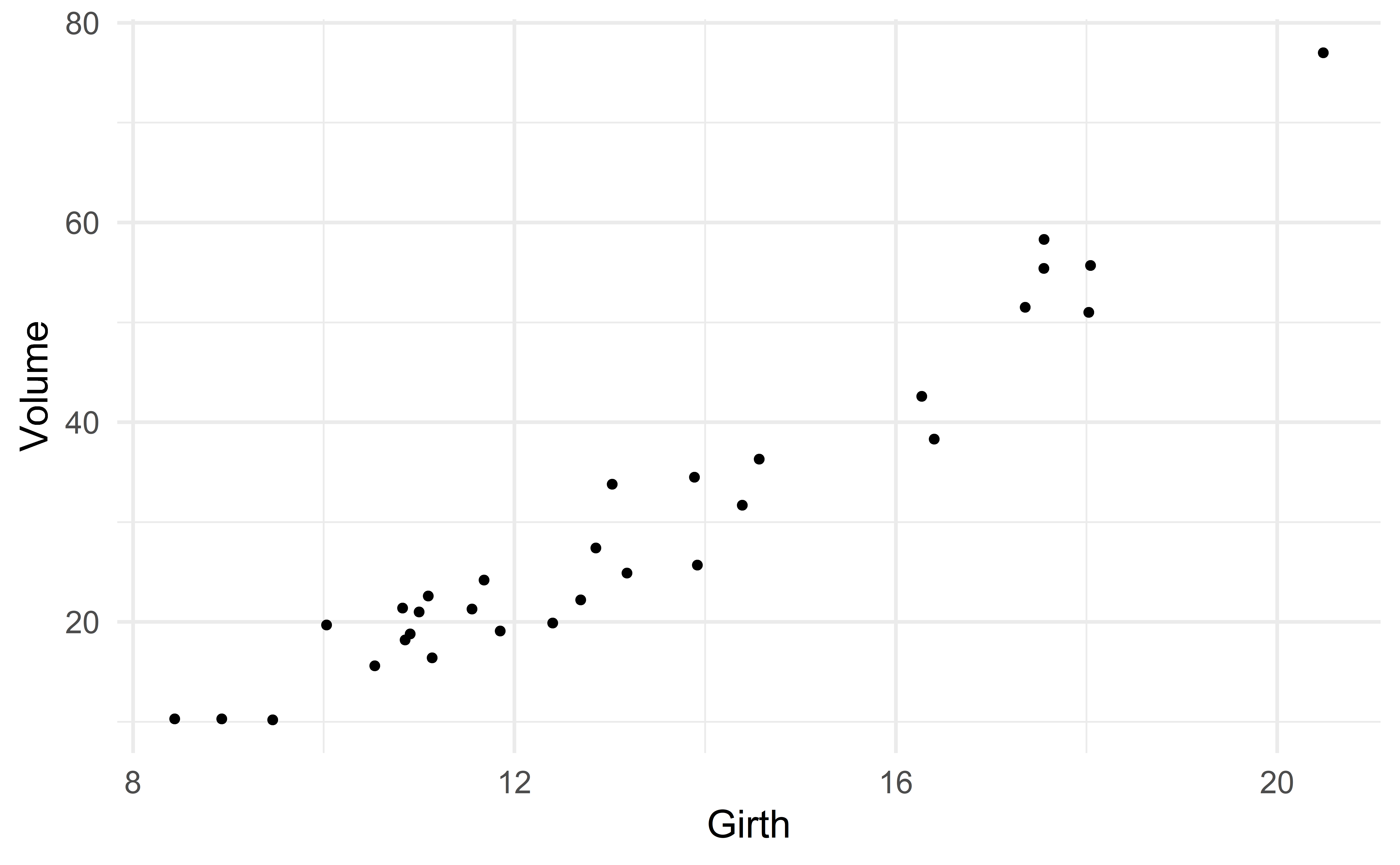
One could argue that there is a slight nonlinear association

Function to compute \(R^2\)

compute_R2 <- function(model){
  
  model_glanced <- glance(model)
  R2 <- model_glanced$r.squared
  R2_rounded <- round(R2, 3) 
  
  return(R2_rounded)
  
}

Starting simple…

We start with the simple model

\[ \text{Volume} \approx \beta_0 + \beta_1 \text{girth} \]

m1 <- lm(Volume ~ Girth, data = d_tree)
compute_R2(m1)

[1] 0.933

• R code
• Regression line

Girth_new <- seq(min(d_tree$Girth), max(d_tree$Girth), by = 0.001)
new_data <- tibble(Girth = Girth_new)
Volume_pred <- predict(m1, new_data)
new_data <- mutate(new_data, Volume_pred = Volume_pred)
head(new_data)

# A tibble: 6 x 2
  Girth Volume_pred
  <dbl>       <dbl>
1  8.44        5.51
2  8.44        5.52
3  8.44        5.52
4  8.44        5.53
5  8.44        5.53
6  8.44        5.54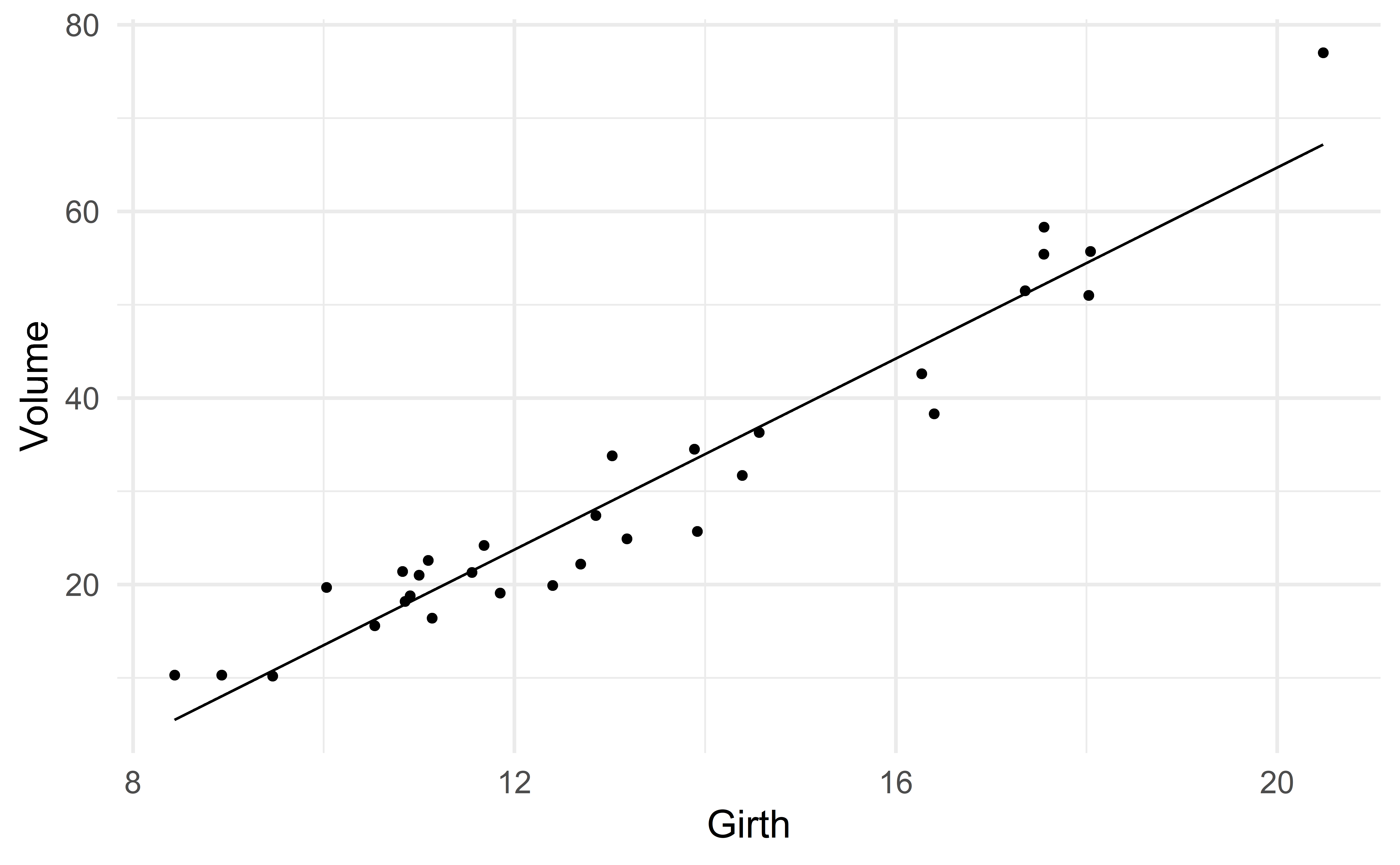

ggplot() +
  geom_point(data = d_tree  , aes(Girth, Volume     )) +
  geom_line (data = new_data, aes(Girth, Volume_pred))

…taking it up a notch…

To capture the nonlinear association between Girth and Volume, we consider the predictor \(\text{Girth}^2\).

\[ \text{Volume} \approx \beta_0 + \beta_1 \text{girth} + \beta_2 \text{girth}^2 \]

The command to fit this model is

d_tree2 <- mutate(d_tree, Girth2 = Girth^2)
m2 <- lm(Volume ~ Girth + Girth2, data = d_tree2)
compute_R2(m2)

[1] 0.958

\(R^2\) has increased! It went from 0.933 (model 1) to 0.958.

• R code
• Regression line

Girth_new <- seq(min(d_tree$Girth), max(d_tree$Girth), by = 0.001)
new_data <- tibble(Girth = Girth_new) %>% mutate(Girth2 = Girth^2)
Volume_pred <- predict(m2, new_data)
new_data <- mutate(new_data, Volume_pred = Volume_pred)
head(new_data)

# A tibble: 6 x 3
  Girth Girth2 Volume_pred
  <dbl>  <dbl>       <dbl>
1  8.44   71.2        11.5
2  8.44   71.2        11.5
3  8.44   71.2        11.5
4  8.44   71.2        11.5
5  8.44   71.2        11.5
6  8.44   71.3        11.5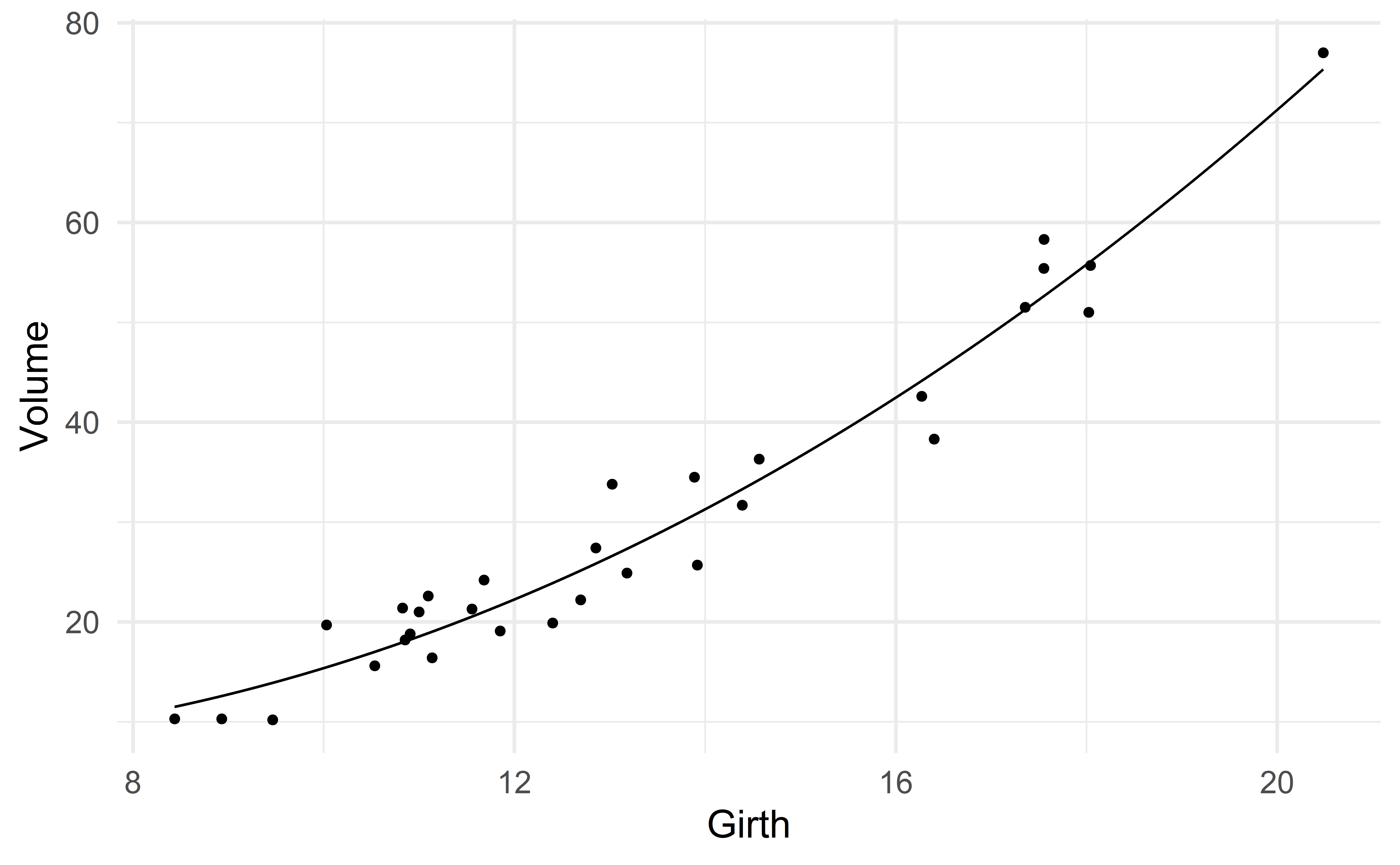

ggplot() +
  geom_point(data = d_tree  , aes(Girth, Volume     )) +
  geom_line (data = new_data, aes(Girth, Volume_pred))

…taking it up another notch…

Let us consider the predictor \(\text{Girth}^3\).

\[ \text{Volume} \approx \beta_0 + \beta_1 \text{girth} + \beta_2 \text{girth}^2 + \beta_3 \text{girth}^3 \]

d_tree3 <- mutate(d_tree, Girth2 = Girth^2, Girth3 = Girth^3)
m3 <- lm(Volume ~ Girth + Girth2 + Girth3, data = d_tree3)
compute_R2(m3)

[1] 0.96

\(R^2\) has increased! It went from 0.958 (model 2) to 0.96.

• R code
• Regression line

Girth_new <- seq(min(d_tree$Girth), max(d_tree$Girth), by = 0.001)
new_data <- tibble(Girth = Girth_new) %>% mutate(Girth2 = Girth^2, Girth3 = Girth^3)
Volume_pred <- predict(m3, new_data)
new_data <- mutate(new_data, Volume_pred = Volume_pred)
head(new_data)

# A tibble: 6 x 4
  Girth Girth2 Girth3 Volume_pred
  <dbl>  <dbl>  <dbl>       <dbl>
1  8.44   71.2   601.        9.83
2  8.44   71.2   601.        9.83
3  8.44   71.2   601.        9.83
4  8.44   71.2   601.        9.84
5  8.44   71.2   601.        9.84
6  8.44   71.3   602.        9.84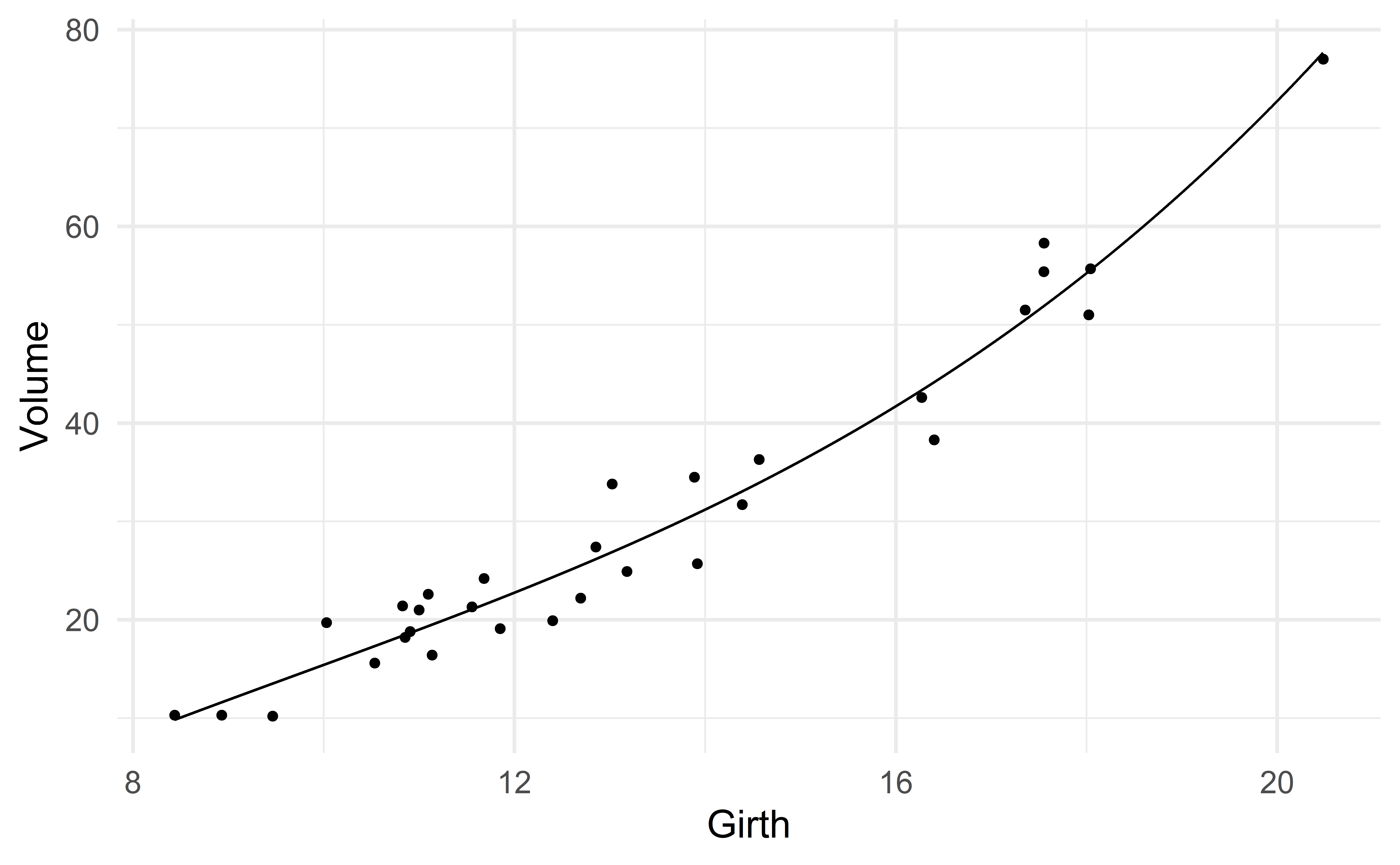

ggplot() +
  geom_point(data = d_tree  , aes(Girth, Volume     )) +
  geom_line (data = new_data, aes(Girth, Volume_pred))

…before taking things to the extreme

What if we also include the predictors \(\text{Girth}^4, \text{Girth}^5, \dots, \text{Girth}^{k}\) for some larger number \(k\)?

The following R command fits the model with \(k=81\), that is,

\[ \text{Volume} \approx \beta_0 + \beta_1 \text{girth} + \beta_2 \text{girth}^2 + \dots + \beta_{81} \text{girth}^{81} \]

m_extreme <- lm(Volume ~ poly(Girth, degree = 81, raw = TRUE), data = d_tree)
compute_R2(m_extreme)

[1] 0.981

\(R^2\) has again increased! It went from 0.96 (model 3) to 0.981.

A limitation of \(R^2\)

As we keep adding predictors, \(R^2\) will always increase.

• additional predictors allow the regression line to be more flexible, hence to be closer to the points and reduce the residuals.

Is the model m_extreme a good model?

Note

We want to learn about the relation between Volume and Girth present in the population (not the sample).

A good model should accurately represent the population.

• R code
• Regression line
• Regression line (zoomed)

Girth_new <- seq(min(d_tree$Girth), max(d_tree$Girth), by = 0.0001)
new_data <- tibble(Girth = Girth_new)
Volume_pred <- predict(m_extreme, new_data)
new_data <- mutate(new_data, Volume_pred = Volume_pred)
head(new_data)

# A tibble: 6 x 2
  Girth Volume_pred
  <dbl>       <dbl>
1  8.44        10.3
2  8.44        10.4
3  8.44        10.4
4  8.44        10.4
5  8.44        10.5
6  8.44        10.5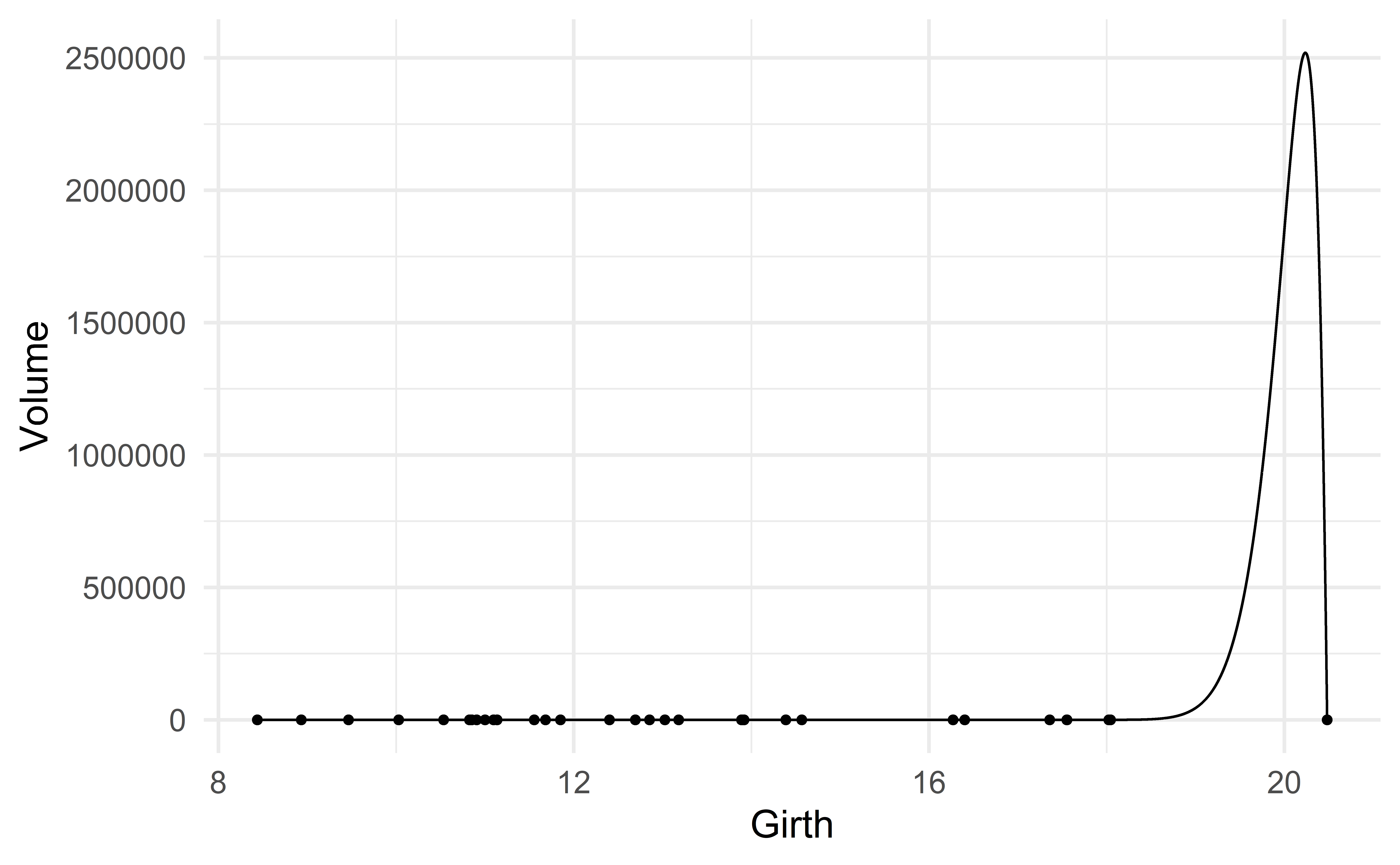

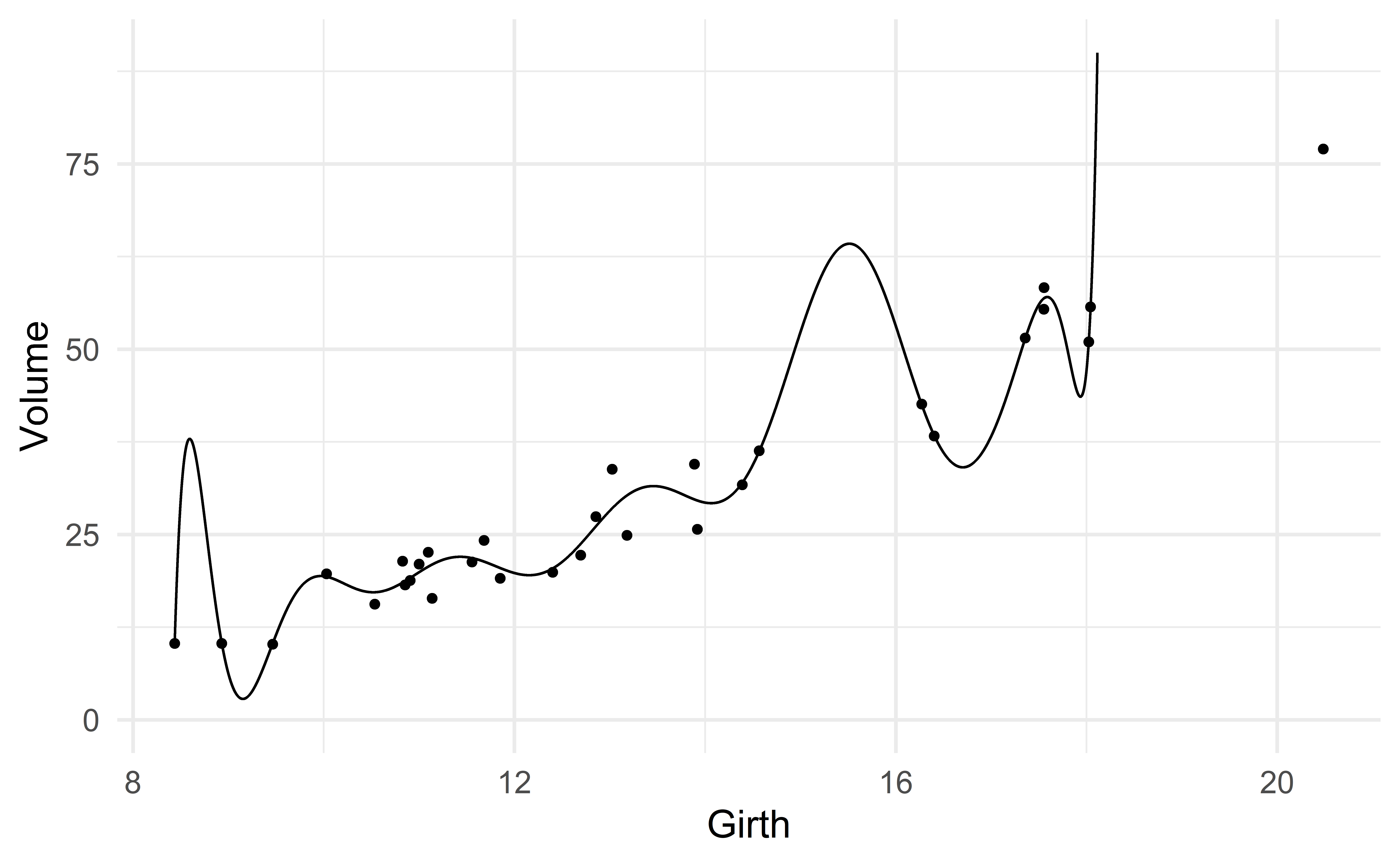
ggplot() +
  geom_point(data = d_tree  , aes(Girth, Volume     )) +
  geom_line (data = new_data, aes(Girth, Volume_pred))

ggplot() +
  geom_point(data = d_tree  , aes(Girth, Volume     )) +
  geom_line (data = new_data, aes(Girth, Volume_pred)) +
  ylim(0, 90)

Overfitting

The model m_extreme overfits the data.

A model overfits the data when it fits the sample extremely well but does a poor job for new data.

Remember that we want to learn about the population, not the sample!

Model selection: overall criteria

\(R^2\)

We saw that \(R^2\) keeps increasing as we add predictors.

\[ R^2 = 1 - \dfrac{SSR}{SST} \]

\(R^2\) can therefore not be used to identify models that overfit the data.

Adjusted-\(R^2\)

The adjusted-\(R^2\) is similar to \(R^2\), but penalizes large models:

\[ R^2_{\text{adj}} = 1 - \dfrac{SSR}{SST}\dfrac{n-1}{n-p-1} \]

where \(p\) corresponds to the number of predictors (model size).

The adjusted-\(R^2\) therefore balances goodness of fit and parsimony:

• The ratio \(\dfrac{SSR}{SST}\) favors model with good fit (like \(R^2\))
• The ratio \(\dfrac{n-1}{n-k-1}\) favors parsimonious models

The model with the highest adjusted-\(R^2\) typically provides a good fit without overfitting.

Group exercise - a function for the adjusted-\(R^2\)

Consider the function compute_R2 which takes a model as input and returns its \(R^2\) rounded to the 3rd decimal.

compute_R2 <- function(model){
  
  model_glanced <- glance(model)
  R2 <- model_glanced$r.squared
  R2_rounded <- round(R2, 3) 
  
  return(R2_rounded)
  
}

Adapt the function so that it computes the adjusted-\(R^2\) instead of \(R^2\). Give an appropriate name to the new function.

04:00

AIC and BIC

Two other popular overall criteria that balance goodness of fit (small SSR) and parsimony (small \(p\)) are

• the Akaike Information Criterion (AIC)
• the Bayesian Information Criterion (BIC)

The formula for AIC and BIC are respectively

\[ AIC = 2p - \text{GoF}, \qquad BIC = \ln(n)p- \text{GoF} \]

where \(\text{GoF}\) measures the goodness of fit of the model¹.

1. The exact formula for \(\text{GoF}\) is beyond the scope of this class.

AIC and BIC in practice

Warning

Unlike the adjusted-\(R^2\), smaller is better for the AIC and BIC.

Note

The BIC penalizes the number of parameters \(p\) more strongly than AIC. BIC will therefore tend to favor smaller models (models with fewer parameters).

Computing AIC and BIC

AIC and BIC are easily accessible in R with the command glance.

rbind(glance(m1), glance(m2), glance(m3), glance(m_extreme))

# A tibble: 4 x 12
  r.squared adj.r.squared sigma statistic  p.value    df logLik   AIC   BIC
      <dbl>         <dbl> <dbl>     <dbl>    <dbl> <dbl>  <dbl> <dbl> <dbl>
1     0.933         0.930  4.34     401.  1.57e-18     1  -88.5  183.  187.
2     0.958         0.955  3.50     317.  5.93e-20     2  -81.3  171.  176.
3     0.960         0.955  3.48     214.  6.39e-19     3  -80.5  171.  178.
4     0.981         0.960  3.28      46.3 2.32e- 9    16  -68.5  173.  199.
# ... with 3 more variables: deviance <dbl>, df.residual <int>, nobs <int>

In this case, BIC favor m2, AIC cannot decide between m2 and m3 and the adjusted-\(R^2\) (wrongly) favors m_extreme.

• For AIC and BIC, smaller is better!
• BIC favors more parsimonious models than AIC.

Model selection: predictive performance

Limitations of the previous criteria

The adjusted-\(R^2\), AIC and BIC all try to balance

1. goodness of fit
2. parsimony

They achieve this balance by favoring models with small SSR while penalizing models with larger \(p\).

…But

• The form of the penalty for \(p\) is somewhat arbitrary, e.g. AIC versus BIC.
• The adjusted-\(R^2\) failed to penalize m_extreme, although it was clearly overfitting the data.

Predictive performance

Instead of using these criteria, we could look for the model with the best predictions performance.

That is, the model that makes predictions for new observations that are the closest to the true values.

We will learn two approaches to accomplish this

• the holdout method
• cross-validation

The holdout method

The holdout method is a simple method to evaluate the predictive performance of a model.

1. Randomly partition your sample into two sets: a training set (typically 2/3 of the sample) and a test set (the remaining 1/3).

2. Fit your model to the training set.

3. Evaluate the prediction accuracy of the model on the test set.

Note that the test set consists of new observations for the model.

\(\Rightarrow\) Select the model with the best prediction accuracy in step 3.

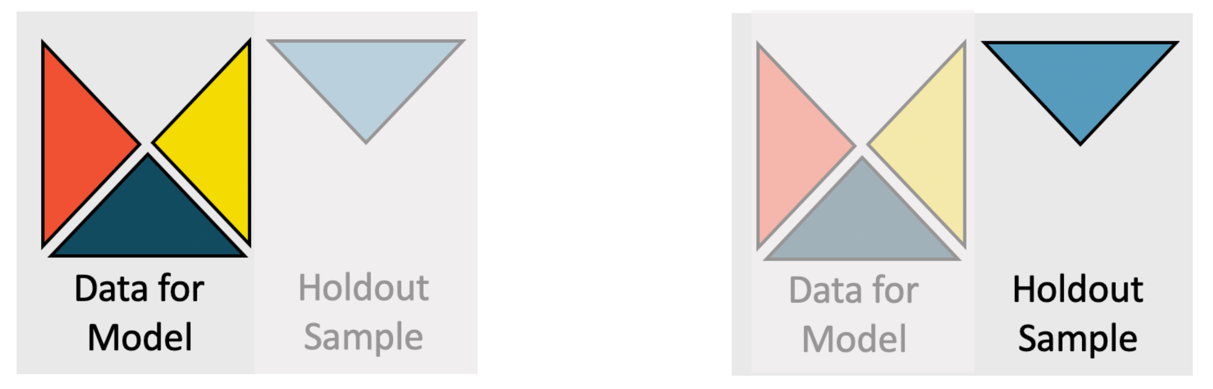
The holdout method.

Source: IMS

Step 1: training and test sets

The following R function splits a sample into a training and a test set

construct_training_test <- function(sample, prop_training = 2/3){
  
  n          <- nrow(sample)
  n_training <- round(n * prop_training)
  
  sample_random   <- slice_sample(sample, n = n)
  sample_training <- slice(sample_random,    1 : n_training )
  sample_test     <- slice(sample_random, - (1 : n_training))
  
  return(list(
    training = sample_training, test = sample_test
    ))
  
}

• Sample
• Training set
• Test set

d_tree # entire sample

       Girth Height Volume
1   8.931477     70   10.3
2   8.436883     65   10.3
3   9.464900     63   10.2
4  11.136215     72   16.4
5  10.907321     81   18.8
6  10.030025     83   19.7
7  10.535716     66   15.6
8  10.852640     75   18.2
9  11.097116     80   22.6
10 12.402327     75   19.9
11 11.681797     79   24.2
12 11.000495     76   21.0
13 10.826171     76   21.4
14 11.555269     69   21.3
15 11.850392     75   19.1
16 12.694245     74   22.2
17 13.026112     85   33.8
18 12.854039     86   27.4
19 13.917842     71   25.7
20 13.181231     64   24.9
21 13.887866     78   34.5
22 14.388698     80   31.7
23 14.566668     74   36.3
24 16.402095     72   38.3
25 16.271447     77   42.6
26 17.551804     81   55.4
27 18.042885     82   55.7
28 17.554523     80   58.3
29 17.357700     80   51.5
30 18.023363     80   51.0
31 20.482147     87   77.0

set.seed(0) # set the seed of the random number generator to 0
training_test_sets <- construct_training_test(d_tree) 
training_set <- training_test_sets[["training"]]
training_set

       Girth Height Volume
1  11.555269     69   21.3
2  16.271447     77   42.6
3  11.136215     72   16.4
4  10.535716     66   15.6
5   8.931477     70   10.3
6   8.436883     65   10.3
7  14.566668     74   36.3
8  11.681797     79   24.2
9  20.482147     87   77.0
10 12.854039     86   27.4
11 13.917842     71   25.7
12 18.042885     82   55.7
13 12.402327     75   19.9
14 18.023363     80   51.0
15 13.887866     78   34.5
16 17.554523     80   58.3
17 11.097116     80   22.6
18 10.907321     81   18.8
19 14.388698     80   31.7
20 11.850392     75   19.1
21 11.000495     76   21.0

test_set <- training_test_sets[["test"]]
test_set

      Girth Height Volume
1  10.82617     76   21.4
2  13.02611     85   33.8
3  17.55180     81   55.4
4  10.85264     75   18.2
5  10.03002     83   19.7
6  13.18123     64   24.9
7  17.35770     80   51.5
8   9.46490     63   10.2
9  16.40209     72   38.3
10 12.69424     74   22.2

Step 2: fit the model to the training set

We simply fit our regression model to the training set.

m1 <- lm(Volume ~ Girth, data = training_set)

Step 3: Evaluate the prediction accuracy on the test set

To evaluate the prediction accuracy, we start by computing the predictions for the observations in the test set.

Volume_hat <- predict(m1, test_set)

A good model will make predictions that are closed to the true values of the response variable.

Sum of squared errors

A good measure of prediction accuracy is the sum of squared errors (SSE).

\[ SSE = (y_1 - \hat{y}_1)^2 + (y_2 - \hat{y}_2)^2 + \dots + (y_m - \hat{y}_m)^2 \]

Small SSE is better.

Volume <- test_set$Volume
sum((Volume - Volume_hat)^2)

[1] 211.4543

Mean squared error

In practice, the (root) mean sum of squared errors ((R)MSE) is often used.

\[ MSE = \dfrac{SSE}{m} = \dfrac{(y_1 - \hat{y}_1)^2 + (y_2 - \hat{y}_2)^2 + \dots + (y_m - \hat{y}_m)^2}{m} \]

\[ RMSE = \sqrt{\dfrac{SSE}{m}} = \sqrt{\dfrac{(y_1 - \hat{y}_1)^2 + (y_2 - \hat{y}_2)^2 + \dots + (y_m - \hat{y}_m)^2}{m}} \] Again, small (R)MSE is better.

SSE <- sum ((Volume - Volume_hat)^2)
MSE <- mean((Volume - Volume_hat)^2)
RMSE <- sqrt(MSE)
SSE; MSE; RMSE

[1] 211.4543

[1] 21.14543

[1] 4.598416

(R)MSE

The advantage of (R)MSE over SSE is that we can compare models that are evaluated with test sets of different sizes.

Selecting a model

Apply steps 2 and 3 on different models.

• use the same training and test sets from step 1 for the different models

\(\Rightarrow\) Choose the model with the lowest (R)MSE!

This model has the best predictive accuracy.

Function to compute the RMSE

compute_RMSE <- function(test_set, model){
  
  y     <- test_set$Volume # truth
  y_hat <- predict(model, test_set) # predicted value
  
  E    <- y - y_hat
  MSE  <- mean(E^2)
  RMSE <- sqrt(MSE)
  
  return(RMSE)
  
}

# Step 1 - partition sample into a training set and a test set
# already done

# Step 2 - fit models to training set
m1  <- lm(Volume ~ poly(Girth, degree = 1 , raw = TRUE), data = training_set)
m2  <- lm(Volume ~ poly(Girth, degree = 2 , raw = TRUE), data = training_set)
m3  <- lm(Volume ~ poly(Girth, degree = 3 , raw = TRUE), data = training_set)
m48 <- lm(Volume ~ poly(Girth, degree = 48, raw = TRUE), data = training_set)

# Step 3 - evaluate models on test set
compute_RMSE(test_set, m1)
compute_RMSE(test_set, m2)
compute_RMSE(test_set, m3) # best
compute_RMSE(test_set, m48)

[1] 4.598416
[1] 4.07333
[1] 3.957379
[1] 29.97533

We select m3.

Limitation of the holdout method

The previous analysis was conducted with set.seed(0).

Note that models m2 and m3 were pretty close.

Could we have obtained a different result with a different seed?

# Step 1
set.seed(1) # new seed
training_test_sets <- construct_training_test(d_tree) 
training_set <- training_test_sets[["training"]]
test_set <- training_test_sets[["test"]]

# Step 2
m1  <- lm(Volume ~ poly(Girth, degree = 1 , raw = TRUE), data = training_set)
m2  <- lm(Volume ~ poly(Girth, degree = 2 , raw = TRUE), data = training_set)
m3  <- lm(Volume ~ poly(Girth, degree = 3 , raw = TRUE), data = training_set)
m48 <- lm(Volume ~ poly(Girth, degree = 48, raw = TRUE), data = training_set)

# Step 3
compute_RMSE(test_set, m1)
compute_RMSE(test_set, m2) # best
compute_RMSE(test_set, m3)
compute_RMSE(test_set, m48)

[1] 6.097541
[1] 4.248172
[1] 10.37698
[1] 103753769

The test set matters!

With set.seed(1), the holdout method indicates that m2 is the best model.

• m3, our previous best model, is worse than m1!

A drawback of the holdout method is that the test set matters a lot.

• Repeating steps 2 and 3 with a different partition in step 1 may give different results.

Group exercise - limitation of the holdout method

Copy and paste the following code in your R session. Try a few different seed numbers for step 1. Keep track of which model has the lowest RMSE. Is m1 ever the best model?

You can safely ignore the warning messages.

# Setup
set.seed(0) # do not change this seed number
d_tree <- datasets::trees %>% mutate(Girth = Girth + rnorm(nrow(.), 0, 0.5))
compute_RMSE <- function(test_set, model){
  
  y     <- test_set$Volume
  y_hat <- predict(model, test_set)
  
  E    <- y - y_hat
  MSE  <- mean(E^2)
  RMSE <- sqrt(MSE)
  
  return(RMSE)
  
}
construct_training_test <- function(sample, prop_training = 2/3){
  
  n          <- nrow(sample)
  n_training <- round(n * prop_training)
  
  sample_random   <- slice_sample(sample, n = n)
  sample_training <- slice(sample_random,    1 : n_training )
  sample_test     <- slice(sample_random, - (1 : n_training))
  
  return(list(
    training = sample_training, test = sample_test
    ))
  
}

# Step 1
set.seed(2) # try a few different seed numbers
training_test_sets <- construct_training_test(d_tree) 
training_set <- training_test_sets[["training"]]
test_set <- training_test_sets[["test"]]

# Step 2
m1  <- lm(Volume ~ poly(Girth, degree = 1 , raw = TRUE), data = training_set)
m2  <- lm(Volume ~ poly(Girth, degree = 2 , raw = TRUE), data = training_set)
m3  <- lm(Volume ~ poly(Girth, degree = 3 , raw = TRUE), data = training_set)
m48 <- lm(Volume ~ poly(Girth, degree = 48, raw = TRUE), data = training_set)

# Step 3
compute_RMSE(test_set, m1)
compute_RMSE(test_set, m2)
compute_RMSE(test_set, m3)
compute_RMSE(test_set, m48)

05:00

Cross-validation

Cross-validation (CV) is a natural generalization of the holdout method:

• repeat the holdout method many times with different partitions in step 1.

0. randomly partition the sample into \(k\) folds of equal size. \(k\) is typically \(5\) or \(10\).

Repeat the following steps \(k\) times

1. Let fold 1 be the test set and the remaining folds be the training set.

2. Fit the model to the training set (like the holdout method)

3. Evaluate the prediction accuracy of the model on the test set (like the holdout method)

4. Go back to step 1, let the next fold be the test set.

\(\Rightarrow\) Select the model with the best overall prediction accuracy in step 3.

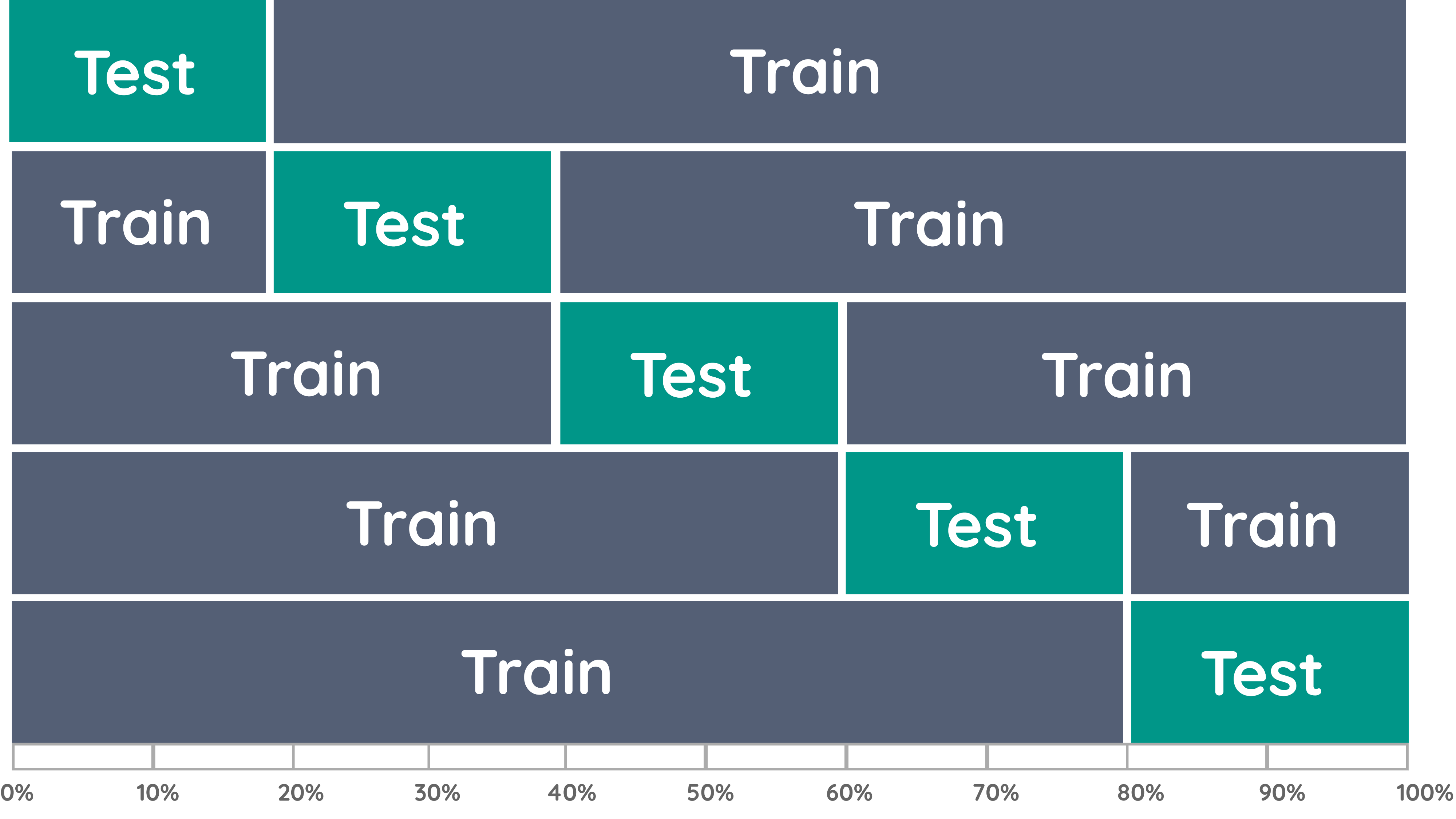
Source: towardsdatascience

Step 0

set.seed(0)

# Setup
n <- nrow(d_tree)
n_folds <- 10

# Fold assignment
folds <- c(rep(1:n_folds, n %/% n_folds), seq_along(n %% n_folds))
# you do not need to understand the details of the previous line
# just note that it creates folds of (almost) the same size
folds

 [1]  1  2  3  4  5  6  7  8  9 10  1  2  3  4  5  6  7  8  9 10  1  2  3  4  5
[26]  6  7  8  9 10  1

# Step 1
d_tree_fold <- d_tree %>%
  slice_sample(n = n) %>% # shuffle the rows
  mutate(fold = folds)
head(d_tree_fold)

      Girth Height Volume fold
1 11.555269     69   21.3    1
2 16.271447     77   42.6    2
3 11.136215     72   16.4    3
4 10.535716     66   15.6    4
5  8.931477     70   10.3    5
6  8.436883     65   10.3    6

Steps 1-4 – Setup

create_empty_RMSE <- function(){
  tibble(
    fold     = numeric(),
    rmse_m1  = numeric(), 
    rmse_m2  = numeric(), 
    rmse_m3  = numeric(), 
    rmse_m48 = numeric()
  )
}

RMSE <- create_empty_RMSE()
RMSE

# A tibble: 0 x 5
# ... with 5 variables: fold <dbl>, rmse_m1 <dbl>, rmse_m2 <dbl>,
#   rmse_m3 <dbl>, rmse_m48 <dbl>

Steps 1-4

RMSE <- create_empty_RMSE()

for(i in 1 : n_folds){
  
  # Step 1
  training_set <- filter(d_tree_fold, fold != i)
  test_set     <- filter(d_tree_fold, fold == i)
  
  # Step 2
  m1  <- lm(Volume ~ poly(Girth, degree = 1 , raw = TRUE), data = training_set)
  m2  <- lm(Volume ~ poly(Girth, degree = 2 , raw = TRUE), data = training_set)
  m3  <- lm(Volume ~ poly(Girth, degree = 3 , raw = TRUE), data = training_set)
  m48 <- lm(Volume ~ poly(Girth, degree = 48, raw = TRUE), data = training_set)
  
  # Step 3
  rmse_m1  <- compute_RMSE(test_set, m1 )
  rmse_m2  <- compute_RMSE(test_set, m2 )
  rmse_m3  <- compute_RMSE(test_set, m3 )
  rmse_m48 <- compute_RMSE(test_set, m48)
  
  RMSE <- RMSE %>% 
    add_row(fold = i, rmse_m1, rmse_m2, rmse_m3, rmse_m48)
  
}

Model selection with RMSE

Which model has the lowest RMSE across all folds?

RMSE

# A tibble: 10 x 5
    fold rmse_m1 rmse_m2 rmse_m3   rmse_m48
   <dbl>   <dbl>   <dbl>   <dbl>      <dbl>
 1     1    5.07    3.50    3.54       4.25
 2     2    2.89    2.34    1.95      10.8 
 3     3    4.78    5.02    5.11       5.54
 4     4    2.82    3.49    3.45       3.15
 5     5    1.67    2.99    2.67      72.5 
 6     6    6.38    4.45    5.38     412.  
 7     7    3.52    2.89    2.83       4.73
 8     8    1.37    2.01    1.77       3.90
 9     9    7.49    3.14    3.92 2481852.  
10    10    5.60    4.53    4.27       4.47

summarise_all(RMSE, mean)

# A tibble: 1 x 5
   fold rmse_m1 rmse_m2 rmse_m3 rmse_m48
  <dbl>   <dbl>   <dbl>   <dbl>    <dbl>
1   5.5    4.16    3.44    3.49  248237.

summarise_all(RMSE, sum ) # what the book uses

# A tibble: 1 x 5
   fold rmse_m1 rmse_m2 rmse_m3 rmse_m48
  <dbl>   <dbl>   <dbl>   <dbl>    <dbl>
1    55    41.6    34.4    34.9 2482374.

m2 has slightly better overall RMSE.

Group exercise - cross-validation

Exercise 25.9, 25.11, 25.12

In part c (25.9 and 25.11) , replace left and right, by top and bottom.

04:00

Short podcast on cross-validation

Cross-validation is a central technique in machine learning.

Still not totally clear how it works? Check out this podcast to hear more about this important topic.

These two other podcasts on muliple linear regression and \(R^2\) are also excellent.

Taking things to the extreme: LOOCV

Set \(k=n\).

• that is, use \(n\) folds, each of size \(1\).

• Each test set will therefore consist of a single observation and the corresponding training set of the remaining \(n-1\) observations.

LOOCV

RMSE <- create_empty_RMSE()

# Step 0
n <- nrow(d_tree)
d_tree_loocv <- mutate(d_tree, folds = 1 : n) # every observation belongs to a different fold 

for(i in 1:n){
  
  # Step 1
  training_set <- filter(d_tree_loocv, folds != i)
  test_set     <- filter(d_tree_loocv, folds == i)
  
  # Step 2
  m1  <- lm(Volume ~ poly(Girth, degree = 1 , raw = TRUE), data = training_set)
  m2  <- lm(Volume ~ poly(Girth, degree = 2 , raw = TRUE), data = training_set)
  m3  <- lm(Volume ~ poly(Girth, degree = 3 , raw = TRUE), data = training_set)
  m48 <- lm(Volume ~ poly(Girth, degree = 48, raw = TRUE), data = training_set)
  
  # Step 3
  rmse_m1  <- compute_RMSE(test_set, m1 )
  rmse_m2  <- compute_RMSE(test_set, m2 )
  rmse_m3  <- compute_RMSE(test_set, m3 )
  rmse_m48 <- compute_RMSE(test_set, m48)
  
  RMSE <- RMSE %>%
    add_row(fold = i, rmse_m1, rmse_m2, rmse_m3, rmse_m48)
  
}

summarize_all(RMSE, mean)

# A tibble: 1 x 5
   fold rmse_m1 rmse_m2 rmse_m3 rmse_m48
  <dbl>   <dbl>   <dbl>   <dbl>    <dbl>
1    16    3.64    3.11    3.12  142697.

Model selection: stepwise procedures

Stepwise procedures

Not my favorite method, but it is widely used.

• Akin the “throw cooked spaghetti to the wall and see what sticks” technique.
• This is what you do when you are clueless about what variables may be good predictors
  • …but then you should probably collaborate with a scientific expert.

Two types of stepwise procedures: (i) forward selection and (ii) backward elimination.

Forward selection

1. Choose an overall criterion that balances GoF (small SSR) and parsimony (small \(p\))

   \(\Rightarrow\) adjusted-\(R^2\), AIC or BIC

2. Start with the empty model \(Y \approx \beta_0\), i.e. the model with no predictor. This is our current model

3. Fit all possible models with one additional predictor.

4. Compute the criterion, say the AIC, of each of these models.

5. Identify the model with the smallest AIC. This is our candidate model.

6. If the AIC of the candidate model is smaller (better) than the AIC of the current model, the candidate model becomes the current model. Go back to step 3.

   If the AIC of the candidate model is larger than the AIC of the current model (no new model improves on the current one), the procedure stops, and we select the current model.

Group exercise - forward selection

Exercise 8.13. In addition, fit the candidate model (a single model) in R with the command lm.

library(openintro)
d <- openintro::births14

05:00

Backward elimination

Similar to forward selection, except that

• We start with the full model.
• We remove one predictor at a time,
• until removing any predictor makes the model worse.

Group exercise - backward elimination

Exercise 8.11. In addition, fit the current and candidate models in R with the command lm.

library(openintro)
d <- openintro::births14

05:00

Forward selection versus backward elimination

Note that forward selection and backward elimination need not agree; they may select different models!

. . .

• What to do in that case? Nobody knows.

How to prevent overfitting?

Parsimony

To obtain a parsimonious model

• use your knowledge of the subject to carefuly choose which variables to consider and construct new ones, and
• implement a model selection procedure.

Recap

Recap

• Overfitting

  • limitations of \(R^2\) for model selection

• Model selection through

  • overall criteria (adjusted-\(R^2\), AIC, BIC)

  • predictive performance (holdout method, cross-validation)

  • stepwise procedure (forward, backward)

You are now fully equipped for the prediction project!

🍀 Good luck! 🍀