Multiple Linear Regression Models

STA 101L - Summer I 2022

Raphael Morsomme

Welcome

Announcements

Find the last person you have not worked with
Prediction project
- teams
- deadlines: May 31 (model and presentation) and June 1 (report)

Project - reading in the data

library(readr)
d <- read_csv("https://rmorsomme.github.io/website/projects/training_set.csv")

Recap

simple linear regression model

\[ \text{hwy} \approx \beta_0 + \beta_1 \text{cty} \]

residuals
least-square estimates
parameter interpretation
model comparison with \(R^2\)
outliers

Outline

multiple linear regression
categorical predictor
feature engineering
- transformation
- combination
- interaction

Multiple linear regression

Remember, to improve our initial model with \((\beta_0, \beta_1) = (1, 1.3)\), we could

find better estimates \(\Rightarrow\) least-square estimates,

use additional predictors \(\Rightarrow\) multiple linear regression models

For instance, to predict hwy we could include multiple variables in our model.

The `mpg` data set

d <- ggplot2::mpg
head(d, n = 4)

# A tibble: 4 x 11
  manufacturer model displ  year   cyl trans      drv     cty   hwy fl    class 
  <chr>        <chr> <dbl> <int> <int> <chr>      <chr> <int> <int> <chr> <chr> 
1 audi         a4      1.8  1999     4 auto(l5)   f        18    29 p     compa~
2 audi         a4      1.8  1999     4 manual(m5) f        21    29 p     compa~
3 audi         a4      2    2008     4 manual(m6) f        20    31 p     compa~
4 audi         a4      2    2008     4 auto(av)   f        21    30 p     compa~

Instead of fitting a model with only cty or only displ, we could fit a linear regression model with both predictors!

Linear regression with 2 predictors

The model equation is

\[ \text{hwy} \approx \beta_0 + \beta_1 \text{cty} + \beta_2 \text{displ} \]

We can find the least-square estimates (minimizing the SSR) with the command lm

lm(hwy ~ cty + displ, data = d)


Call:
lm(formula = hwy ~ cty + displ, data = d)

Coefficients:
(Intercept)          cty        displ  
    1.15145      1.32914     -0.03432

which give the following regression equation

\[ \text{hwy} \approx 1.15 + 1.33 \text{cty} - 0.034 \text{displ} \]

Interpretation

Interpreting \(\hat{\beta}_1 = 1.33\):
- “Keeping displ constant, for each additional unit in cty, we would expect hwy to be higher, on average, by 1.33 units.”

Interpreting \(\hat{\beta}_2 = -0.034\):
- “Keeping cty constant, for each additional unit in displ, we would expect hwy to be lower, on average, by 0.034 unit.”

Interpreting \(\hat{\beta}_0 = 1.15\):
- “For a car with cty and displ equal to 0, we would expect hwy to be 1.15.”
- meaningless in this context.

Special case: categorical predictor

In a regression model, categorical predictors are represented using indicator variables.

To represent a categorical predictor with \(k\) levels (categories), we use \((k-1)\) indicator variables¹.

Including `drv`

For instance, the categorical variable drv has \(k=3\) levels (4, f and r), so we can represent it with \(3-1=2\) indicator variables with the following model equation

\[ \text{hwy} \approx \beta_0 + \beta_1 \text{drv_f} + \beta_2 \text{drv_r} \]

Tip

For a binary variable \(k=2\), so we only need \(k-1=1\) indicator variable.

For instance, to include the binary variable year_binary, we only added a single indicator variable to the model.

Using categorical predictors in `R`

lm(hwy ~ drv, data = d)


Call:
lm(formula = hwy ~ drv, data = d)

Coefficients:
(Intercept)         drvf         drvr  
     19.175        8.986        1.825

The model equation with the least-square estimates is

\[ \text{hwy} \approx 19.175 + 8.986 \text{drv_f} + 1.825 \text{drv_r} \]

Interpreting the output

\[ \text{hwy} \approx 19.175 + 8.986 \text{drv_f} + 1.825 \text{drv_r} \]

If a new vehicle has a drv that is:

4, then the two indicator variables drv_f and drv_r take the value 0, and the prediction is \(\widehat{hwy} = 19.175\)

f, then the indicator variables drv_f takes the value 1 and drv_r the value 0, and the prediction is \(\widehat{hwy} = 19.175 + 8.986 = 28.161\)

r, then the indicator variables drv_f takes the value 0 and drv_r the value 1, and the prediction is \(\widehat{hwy} = 19.175 + 1.825 = 21\)

The level (category) 4 is called the reference (baseline) level.

Group exercise - categorical predictor

Exercises 8.5, 8.7
In addition
1. identify the baseline level of the categorical variable in each model.
```
library(openintro)
d <- openintro::births14
```
1. fit the first model in R

05:00

Fitting a larger model

Let us fit a model with cty, drv and disp

m_larger <- lm(hwy ~ cty + drv + displ, data = d)
m_larger


Call:
lm(formula = hwy ~ cty + drv + displ, data = d)

Coefficients:
(Intercept)          cty         drvf         drvr        displ  
      3.424        1.157        2.158        2.360       -0.208

Its \(R^2\) is 0.938.

glance(m_larger)$r.squared

[1] 0.9384357

Unsurprisingly, including additional predictors makes the regression line closer to the points \(\Rightarrow\) residuals are smaller \(\Rightarrow\) SSR is smaller \(\Rightarrow\) \(R^2\) is larger.

Group exercise - computing \(R^2\) by hand

What is the formula for \(R^2\)?
Compute \(R^2\) by hand in R (do not use glance). You can use the following code.

d <- ggplot2::mpg
m_larger <- lm(hwy ~ cty + drv + displ, data = d)
m_augment <- augment(m_larger)

04:00

Fitting the full¹ model

m_full <- lm(
  hwy ~ manufacturer + displ + year + cyl + trans + drv + cty + fl + class,
  data = d
  )

Thanks to the additional predictors, the residuals are very small, making \(R^2\) close to \(1\).

glance(m_full)$r.squared

[1] 0.9773386

Large \(R^2\)

seems great!
…but we will see in the next lecture that this is not always a good sign.

Group exercise - multiple linear regression

Exercise 8.9

fit the model in R
identify the type of each variable
identify the baseline level of the categorical predictors
do parts a-d

library(openintro)
d_birth <- openintro::births14

05:00

Statistics as an art – feature engineering

Feature engineering

We saw that adding predictors to the model seems to help.

However, the variables included in the data set, e.g. displ, year, etc, may not be the most useful predictors for hwy.

Feature engineering refers to the creation of new predictors from the raw variables.

Tip

This is where your understanding of the data, scientific knowledge and experience make a big difference.

Transforming a variable

Nonlinearity

Consider the relation between the predictor displ and the response hwy

ggplot(d) +
  geom_point(aes(displ, hwy))

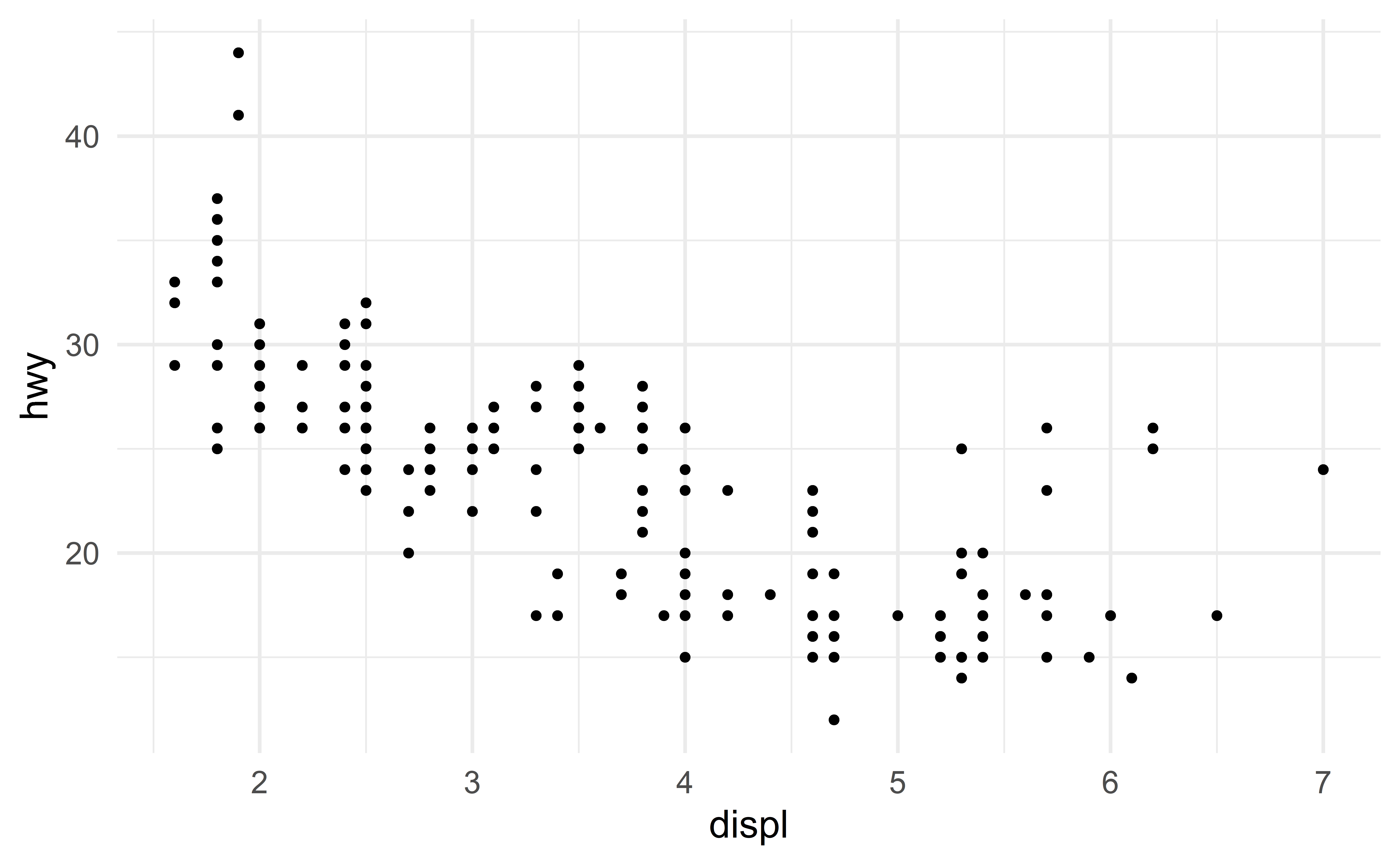
The relationis not exactly linear.

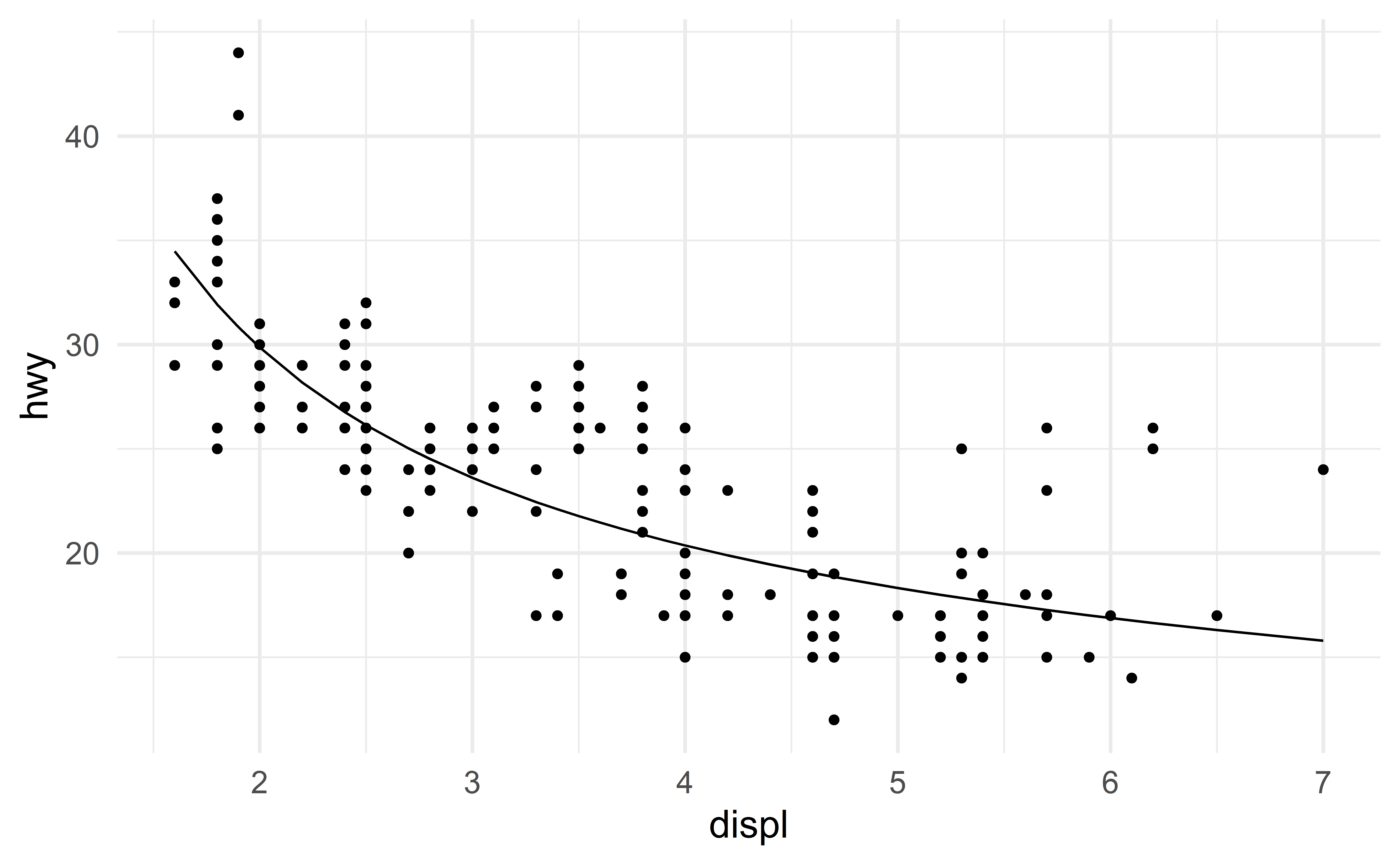
Modeling nonlinearity

Let us include the predictor \(\dfrac{1}{\text{displ}}\) to capture this nonlinear relation.

Here is the model equation

\[ \text{hwy} \approx \beta_0+ \beta_1 \text{displ} + \beta_2 \dfrac{1}{\text{displ}} \]

The least-square coefficient estimates are

d_transf <- mutate(d, displ_inv = 1/displ)
m <- lm(hwy ~ displ + displ_inv, data = d_transf)
m


Call:
lm(formula = hwy ~ displ + displ_inv, data = d_transf)

Coefficients:
(Intercept)        displ    displ_inv  
    12.2601      -0.2332      36.1456

And the regression lines captures the nonlinear relation.

augment(m) %>%
  ggplot(aes(displ, hwy)) +
  geom_point() +
  geom_line(aes(y = .fitted))

Combining variables

The `trees` data set

Measurements of the diameter, height and volume of timber in 31 felled black cherry trees.
Note that the diameter (in inches) is erroneously labelled Girth in the data
The diameter (Girth) is measured at 4 ft 6 in above the ground.
Source: Atkinson, A. C. (1985) Plots, Transformations and Regression. Oxford University Press.

Combining variables

Transforming a variable may be helpful …but we can go a step further!

We can construct new predictors by combining existing variables.

Consider the trees dataset

d_tree <- datasets::trees
head(d_tree, n = 4)

  Girth Height Volume
1   8.3     70   10.3
2   8.6     65   10.3
3   8.8     63   10.2
4  10.5     72   16.4

where Girth indicates the tree diameter (twice the radius) in inches.

Geomtric considerations

Suppose we want to estimate Volume (expensive to measure) from Girth and Height (cheap to measure).

You might decide to approximate the shape of a tree with a shape that is between a cylinder and a cone.

From geometry, we know that the volume of a cylinder is

\[ V = \pi r^2 h \]

and that of a cone is

\[ V = \frac{1}{3} \pi r^2 h \]

This suggests approximating the volume of a tree with the following model

\[ \text{Volume} = \beta_1 \left[ \left(\dfrac{\text{Girth}}{2}\right)^2 * \text{Height}\right] = \beta_1X \]

where

\(\beta_1\) is an unknown parameter that we expect to be between \(\pi\) (pure cylinder) and \(\frac{1}{3}\pi\) (pure cone)
\(X = \left[\left(\dfrac{\text{Girth}}{2}\right)^2 * \text{Height}\right]\) is our new predictor.

To accomplish this, we simply create a new variable corresponding to \(\left[\left(\dfrac{\text{Girth}}{2}\right)^2 * \text{Height}\right]\).

Before doing that, we just need to transform Girth into feet to ensure that all variables have the same units.

d_tree_comb <- d_tree %>%
  mutate(
    Girth_ft    = Girth / 12,
    radius      = Girth_ft / 2,
    r_squared   = radius^2,
    r2h = r_squared * Height
  )
head(d_tree_comb, n = 3)

  Girth Height Volume  Girth_ft    radius r_squared      r2h
1   8.3     70   10.3 0.6916667 0.3458333 0.1196007 8.372049
2   8.6     65   10.3 0.7166667 0.3583333 0.1284028 8.346181
3   8.8     63   10.2 0.7333333 0.3666667 0.1344444 8.470000

Our model does not include an intercept. To exclude the intercept from the model, I use -1 in the lm command.

m_engineered <- lm(Volume ~ r2h - 1, data = d_tree_comb)
m_engineered


Call:
lm(formula = Volume ~ r2h - 1, data = d_tree_comb)

Coefficients:
  r2h  
1.214

The coefficient estimate is between the two anticipated bounds \(\pi=3.14\) and \(\frac{\pi}{3}=1.047\)!

Warning

When we do not include the intercept in a model, \(R^2\) measures something different and should therefore not be interpreted in the usual way.

glance(m_engineered)$r.squared

[1] 0.9950219

Comparison with the full model

Although \(R^2\) has a different meaning when there is no intercept, it can be still used for comparison¹.

m_full <- lm(Volume ~ Girth + Height -1, data = d_tree)
glance(m_full)$r.squared

[1] 0.9696913

glance(m_engineered)$r.squared

[1] 0.9950219

Our new variable \((\dfrac{\text{Girth}}{2})^2 * \text{Height}\) improves the model!

Note that the full model has two predictors, while our geometry-based model has only a single predictor!

Feature engineering

A carefully constructed predictor can do a better job than multiple raw predictors!

Special case of data combination: interaction

Predicting amateur jogging races duration

Suppose you are interested in predicting the average run time (duration) of amateur jogging races.

Two variables that impact the duration are (i) the distance of the race, and (ii) the weather.

For simplicity, we measure the weather as either good (nice weather) or bad (rain, heat wave, etc).

Fixed effect weather?

Te full model is

\[ \text{duration} \approx \beta_0 + \beta_1 \text{distance} + \beta_2 \text{weather_bad} \]

where \(\beta_1\) indicate the effect of an additional miles on the expected duration and \(\beta_2\) the effect of bad weather.

Note that the effect of weather is fixed in this model, say “\(+5\) minutes” if \(\hat{\beta}_2 = 5\).

Is this reasonable? No!

\(\Rightarrow\) the effect of weather should vary with distance. For shorter races, bad weather may add only 2 or 3 minutes, while for longer races, bad weather may increase the average duration by 10 or 15 minutes.

Model equation with interaction

We capture such pattern using an interaction term.

\[ \text{duration} \approx \beta_0 + \beta_1 \text{distance} + \beta_2 \text{weather_bad} + \beta_3 \text{weather_bad}*\text{distance} \]

When the weather is good, the equation simplifies to

\[ \text{duration} \approx \beta_0 + \beta_1 \text{distance} + \beta_2 0 + \beta_3 0*\text{distance} = \beta_0 + \beta_1 \text{distance} \]

When the weather is bad, the equation simplifies to

\[ \text{duration} \approx \beta_0 + \beta_1 \text{distance} + \beta_2 1 + \beta_3 1*\text{distance} = (\beta_0 + \beta_2) + (\beta_1+\beta_3) \text{distance} \]

Interpreting interactions

When the weather is good, the slope estimate is \(\hat{\beta}_1\), meaning that the effect of an additional miles on the average duration is \(\hat{\beta}_1\).
When the weather is bad, the slope estimate is \(\hat{\beta}_1+\hat{\beta}_3\), meaning that the effect of an additional miles on the average duration is \(\hat{\beta}_1+\hat{\beta}_3\) (not \(\hat{\beta}_1\)).

Interactions

The effect of the distance depends on the weather. Similarly, the effect of the weather depends on the distance.

\(\Rightarrow\) the two variables interact.

Recap

simple linear regression model \[ Y \approx \beta_0 + \beta_1 X \]
multiple linear regression model \[ Y \approx \beta_0 + \beta_1 X_1 + \beta_2 X_2 + \dots + + \beta_p X_p \]
categorical predictor
- \((k-1)\) indicator variables
feature engineering
- transforming variables
- combining variables
- interactions

Multiple Linear Regression Models

Welcome

Announcements

Project - reading in the data

Recap

Outline

Multiple linear regression

The mpg data set

Linear regression with 2 predictors

Interpretation

Special case: categorical predictor

Including drv

Using categorical predictors in R

Interpreting the output

Fitting a larger model

Fitting the full1 model

Statistics as an art – feature engineering

Feature engineering

Transforming a variable

Nonlinearity

Modeling nonlinearity

Combining variables

The trees data set

Combining variables

Geomtric considerations

Comparison with the full model

Special case of data combination: interaction

Predicting amateur jogging races duration

Fixed effect weather?

Model equation with interaction

Interpreting interactions

Recap

Recap

The `mpg` data set

Including `drv`

Using categorical predictors in `R`

Fitting the full¹ model

The `trees` data set