Simple Linear Regression Models

STA 101L - Summer I 2022

Raphael Morsomme

Welcome

Announcements

Find someone you have not worked with yet.
Homework 1 has been released
- Ask us if anything is unclear
- regrade window of 48 hours.
Homework 2 has been published
- Due on Wednesday (tomorrow)
- Feel free to re-use the template from HW 1
- There should be no need for external code – look in the lab!

Recap of last lecture

Histogram, scatterplot, boxplot
Average, median, variance, sd and IQR; robustness
Frequency, contigency and proportion tables
Barplot, mosaic plot
Effective communication: well-edited figures, \(\ge3\) variables (symbols, colors, facets)
R for Data Science - chapters 3 and 7

Outline

simple linear regression model
least-square estimates
model comparison
outliers

Simple linear regression

Regression model

d <- ggplot2::mpg
head(d, n = 4)

# A tibble: 4 x 11
  manufacturer model displ  year   cyl trans      drv     cty   hwy fl    class 
  <chr>        <chr> <dbl> <int> <int> <chr>      <chr> <int> <int> <chr> <chr> 
1 audi         a4      1.8  1999     4 auto(l5)   f        18    29 p     compa~
2 audi         a4      1.8  1999     4 manual(m5) f        21    29 p     compa~
3 audi         a4      2    2008     4 manual(m6) f        20    31 p     compa~
4 audi         a4      2    2008     4 auto(av)   f        21    30 p     compa~

Suppose the variable hwy (fuel efficiency on highway) is very expensive to measure.

We decide to estimate it using the other variables. To do so, we will fit a regression model.

\[ \text{hwy} \approx \text{model}(\text{other variables}) \]

Simple regression

We expect the variable cty to be a good proxy for hwy.

After all, if a car is efficient in the city, we expect it to also be efficient on the highway! We will therefore consider a simple regression model

\[ \text{hwy} \approx \text{model}(\text{cty}) \] Simple here means that we include a single predictor in the model.

Simple linear regression

ggplot(d) +
  geom_point(aes(x = cty, y = hwy))

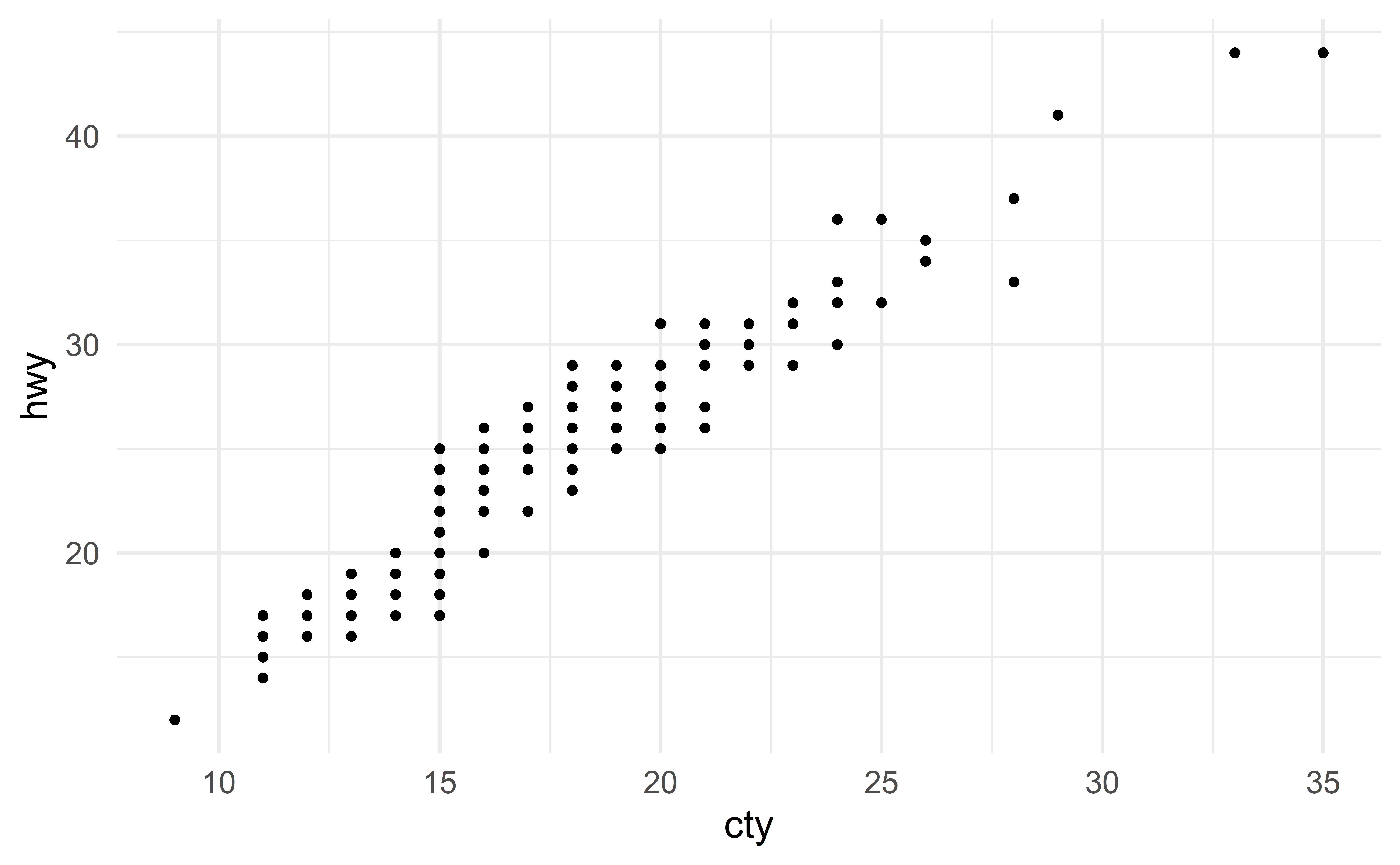
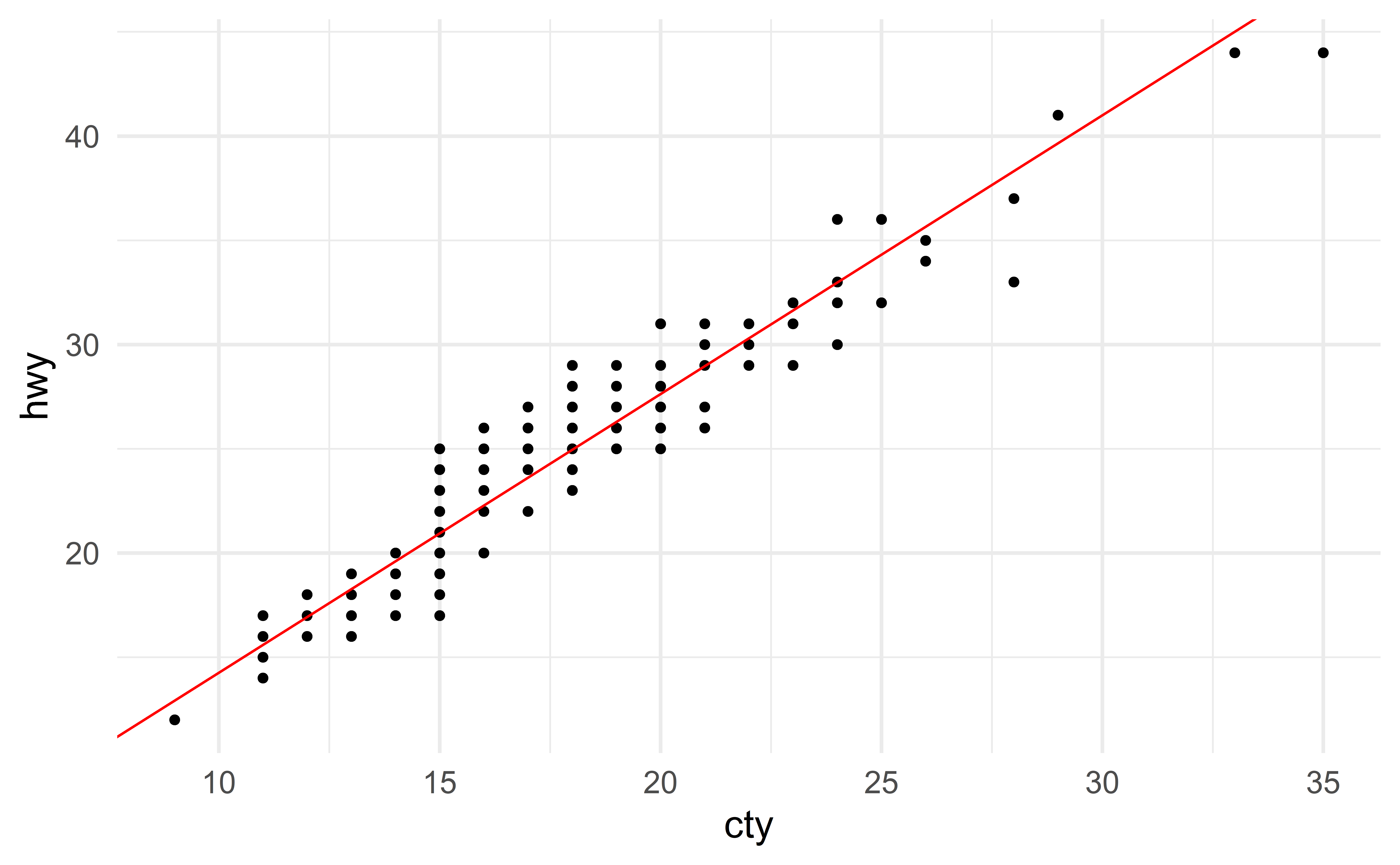
The variables cty and hwy are linearly associated.

We therefore opt for a simple linear regression model

\[ \text{hwy} \approx \beta_0 + \beta_1 \text{cty} \]

Parameters

The numbers \(\beta_0\) and \(\beta_1\) are the two parameters of the model.

We now want to find good values for these unknown parameters.

Let us look at two sets of values:

\[\begin{align*} \beta_0 = 1, \beta_1 = 1.3 \qquad & \Rightarrow \qquad \text{hwy} \approx 1 + 1.3 \text{cty} \\ \beta_0 = 15, \beta_1 = 0.5 \qquad & \Rightarrow \qquad \text{hwy} \approx 15 + 0.5 \text{cty} \end{align*}\]

Good model
Bad model

ggplot(d) +
  geom_point(aes(x = cty, y = hwy)) +
  geom_abline(intercept = 1, slope = 1.3)

ggplot(d) +
  geom_point(aes(x = cty, y = hwy)) +
  geom_abline(intercept = 15, slope = 0.5)

Prediction

We can use our models to estimate hwy for new vehicles.

Imagine there is a new vehicle with \(\text{cty} = 30\). Instead of measuring its hwy (expensive), we use our model to estimate it. Using the “good” model gives the following estimate

\[ \begin{align*} \text{hwy} & \approx \beta_0 + \beta_1 \text{cty} \\ & = 1 + 1.3 * 30\\ & = 40 \end{align*} \]

Is this the true hwy of the new vehicle? No!

this is only an estimate based on the value of the variable cty and our “good” model.

Can we do better? Yes!

Take additional variables into account in the model (e.g. engine size, vehicle age, etc)

Use better values for \(\beta_0\) and \(\beta_1\).

Group exercise - parameters

What is the prediction for the new vehicle (\(\text{cty} = 30\)) if we use the bad model (\(\beta_0 = 15, \beta_1=0.5\))?
Copy and paste the following piece of code and try different values for the parameters to find a good set of values.

library(tidyverse)
d <- ggplot2::mpg
beta_0 <- 15
beta_1 <- 0.5
ggplot(d) +
  geom_point(aes(x = cty, y = hwy)) +
  geom_abline(intercept = beta_0, slope = beta_1)

05:00

Linear association

A simple linear regression model is only applicable if the relation between the predictor and the response is linear.

If the relation is not linear, the simple linear regression is not suitable.

In this case, we need to model the non-linearity (next lecture).

Group exercise - linear association

Exercise 7.3

03:00

Leat-square estimates

Residuals

Our predictions are only approximate.

Let us represent our prediction with \(\widehat{\text{hwy}}\) and the true value with \(\text{hwy}\)
the error we make is \(\text{hw} - \widehat{\text{hwy}}\)
this is called the residual

\[e = \text{hwy} - \widehat{\text{hwy}}\]

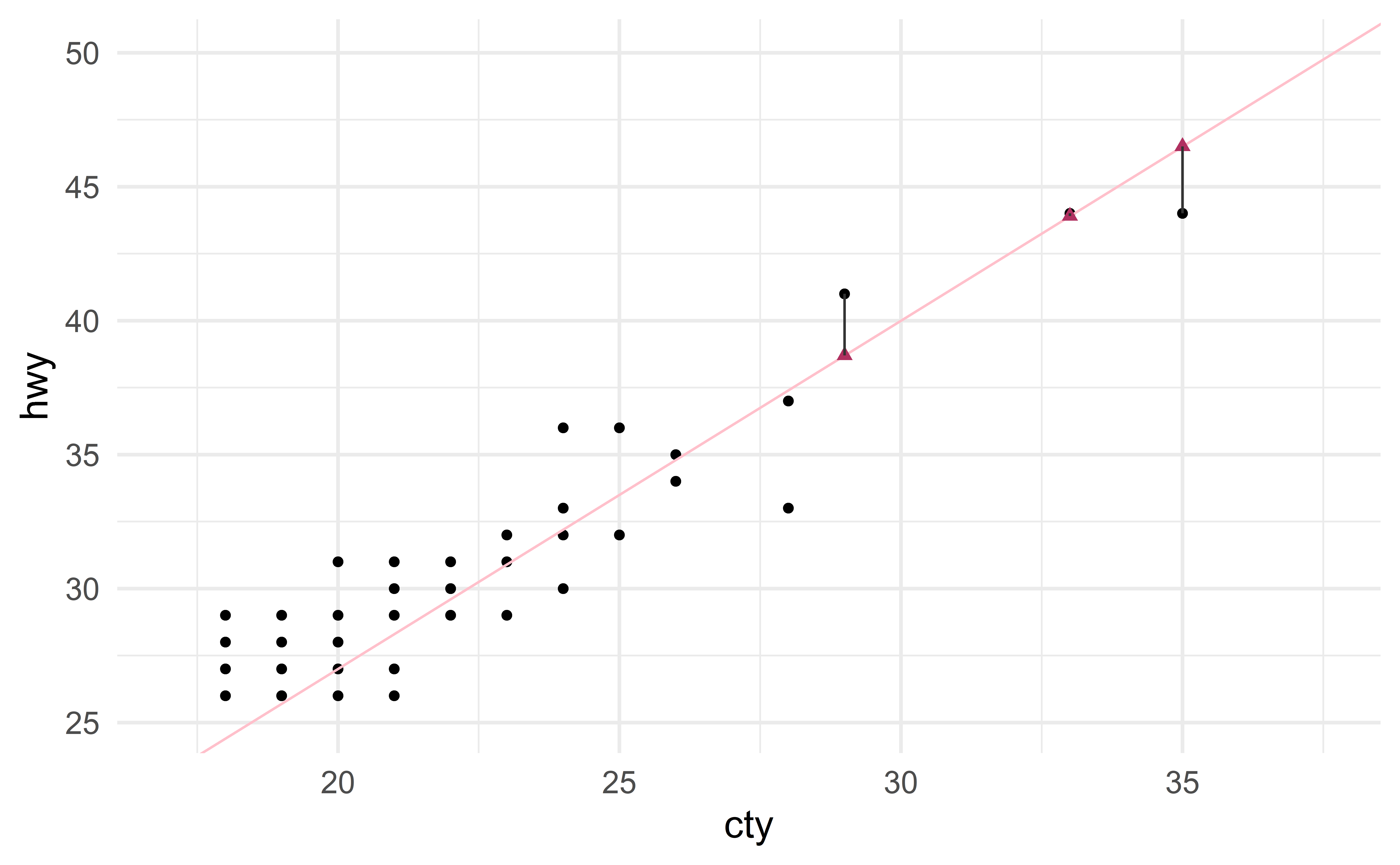
Visualizing residuals

Black circles: Observed values (\(\text{hwy}\))
Pink solid line: Least-squares regression line
Maroon triangles: Predicted values (\(\widehat{\text{hwy}}\))
Gray lines: Residuals

Residual plot

d %>%
  mutate(
    hwy_hat = 1 + 1.3 * cty, # prediction
    resid   = hwy - hwy_hat  # residual
    ) %>%
  ggplot() +
  geom_point(aes(cty, resid)) +
  geom_abline(intercept = 0, slope = 0, col = "red")

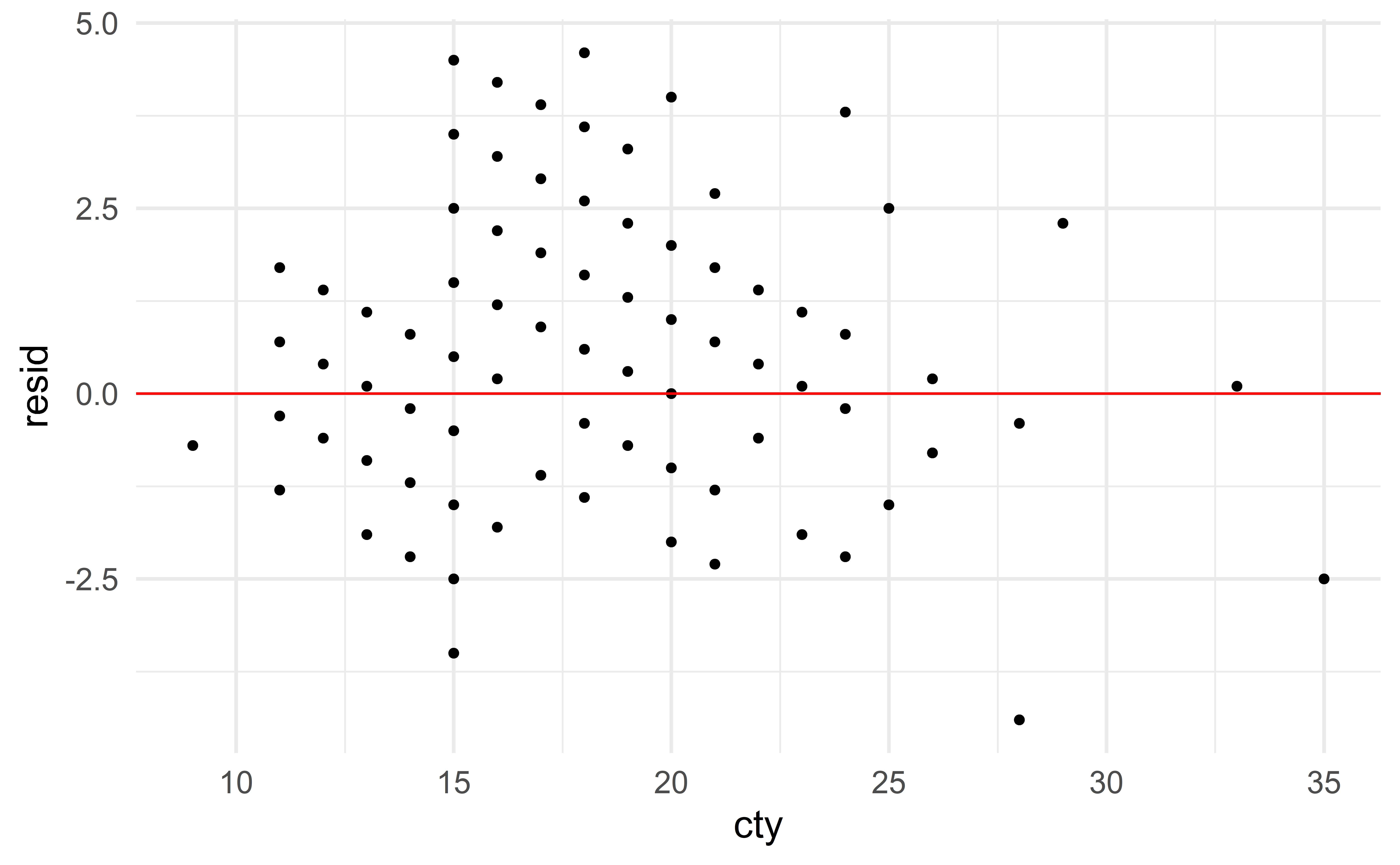
Assessing linearity with residual plots

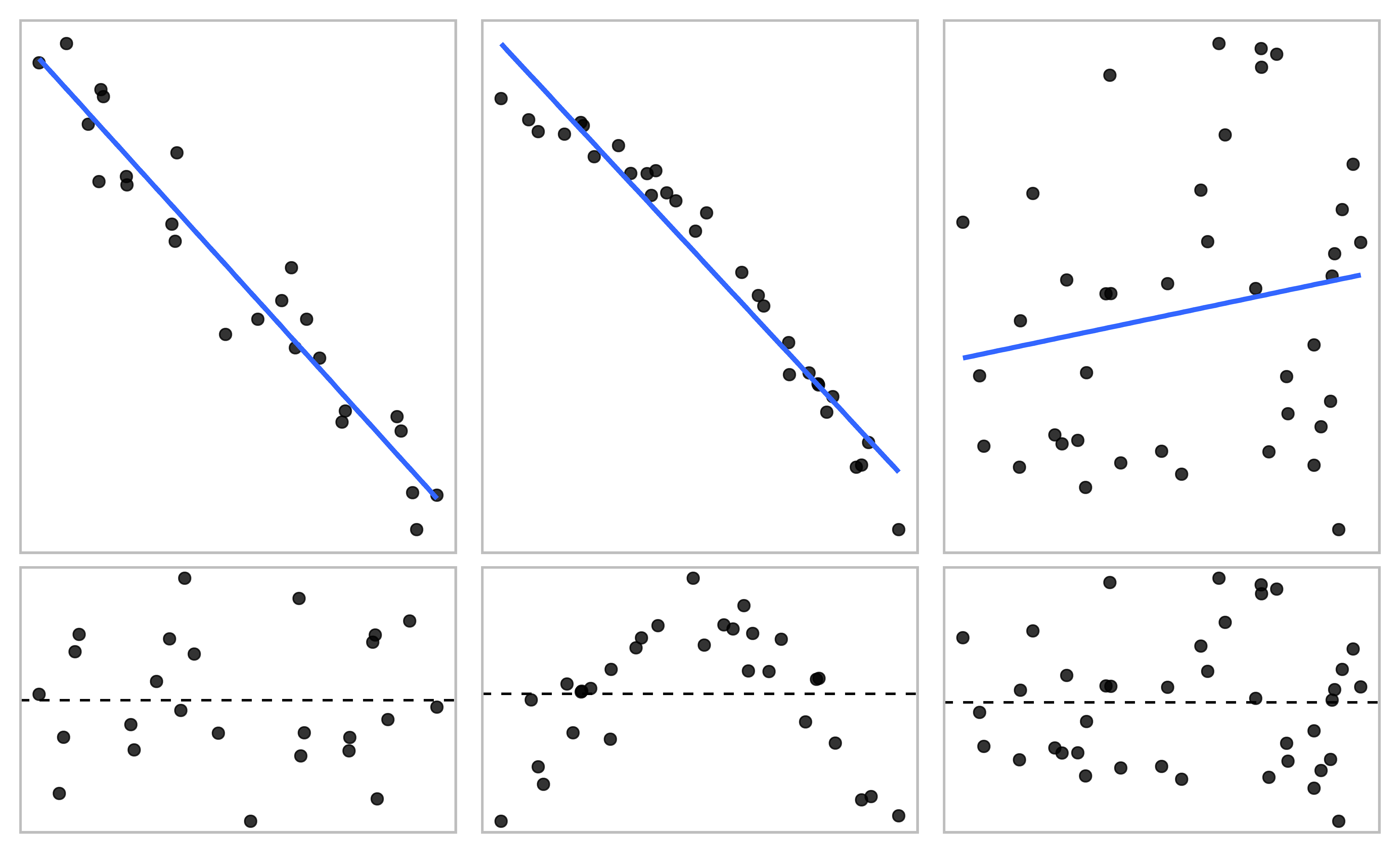
Source: IMS

Group exercise - residuals

Exercises 7.1, 7.17, 7.19

05:00

Good estimates

We want to choose estimates that give a model that fits the data well.

a model with a regression line that is close to the data

We want to minimize the residuals.

Minimizing residuals

Perhaps the most natural thing to do is to find the values of \(\beta_0\) and \(\beta_1\) that minimize the sum of absolute residuals

\[ |e_1|+|e_2|+\dots+|e_n| \]

For practical reasons, the sum of squared residuals (SSR) is a more common criterion

\[ e_1^2+e_2^2+\dots+e_n^2 \]

Why squaring the residuals?

nice mathematical properties
- can work by hand (pre-computer era; first derived by Gauss in the late 1700s (Stigler, 1981))
reflects the assumptions that being off by \(4\) is more than twice as bad as being off by \(2\)
mainstream, e.g. the command lm in R.

Least-square estimates

We simply find the values for \(\beta_0\) and \(\beta_1\) that minimize the SSR with the R command lm

m <- lm(hwy ~ cty, data = d) # find least-square estimates
m


Call:
lm(formula = hwy ~ cty, data = d)

Coefficients:
(Intercept)          cty  
      0.892        1.337

The symbols \(\hat{\beta}_0\) and \(\hat{\beta}_1\) denote least-square estimates.

In our model, we therefore have \[\hat{\beta}_0 = 0.892, \qquad \hat{\beta}_1 = 1.337\]

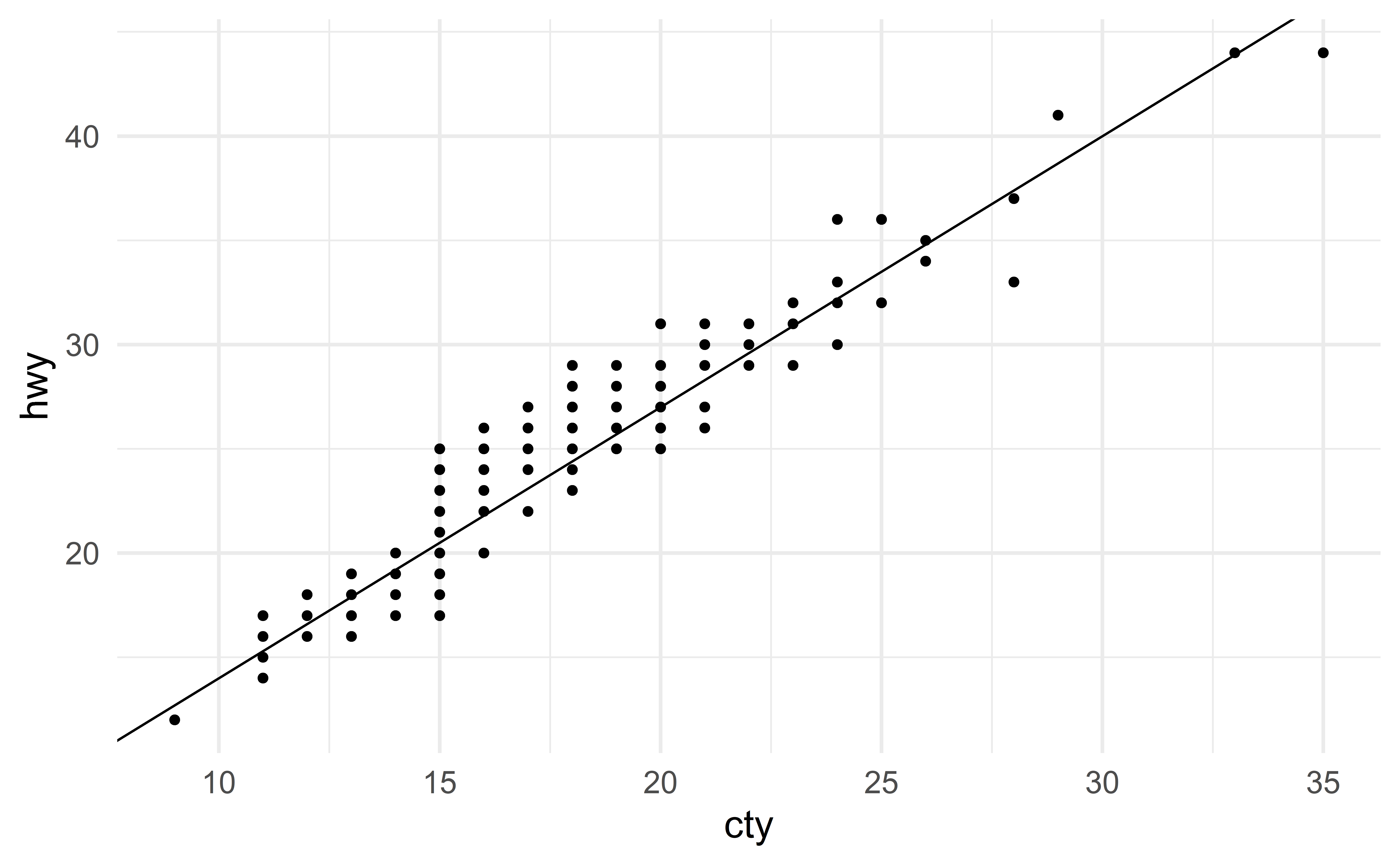
Visualizing the least square regression line

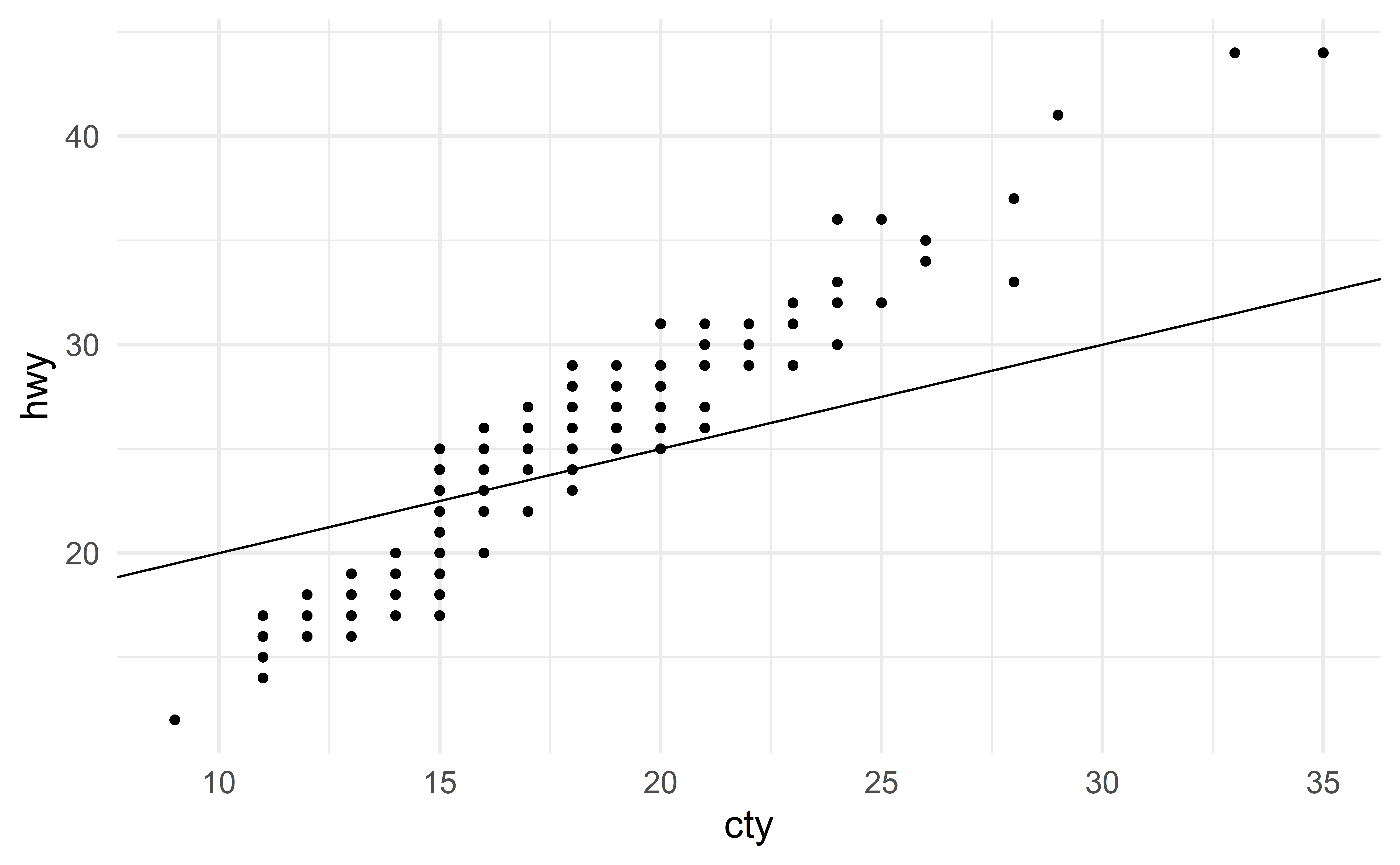
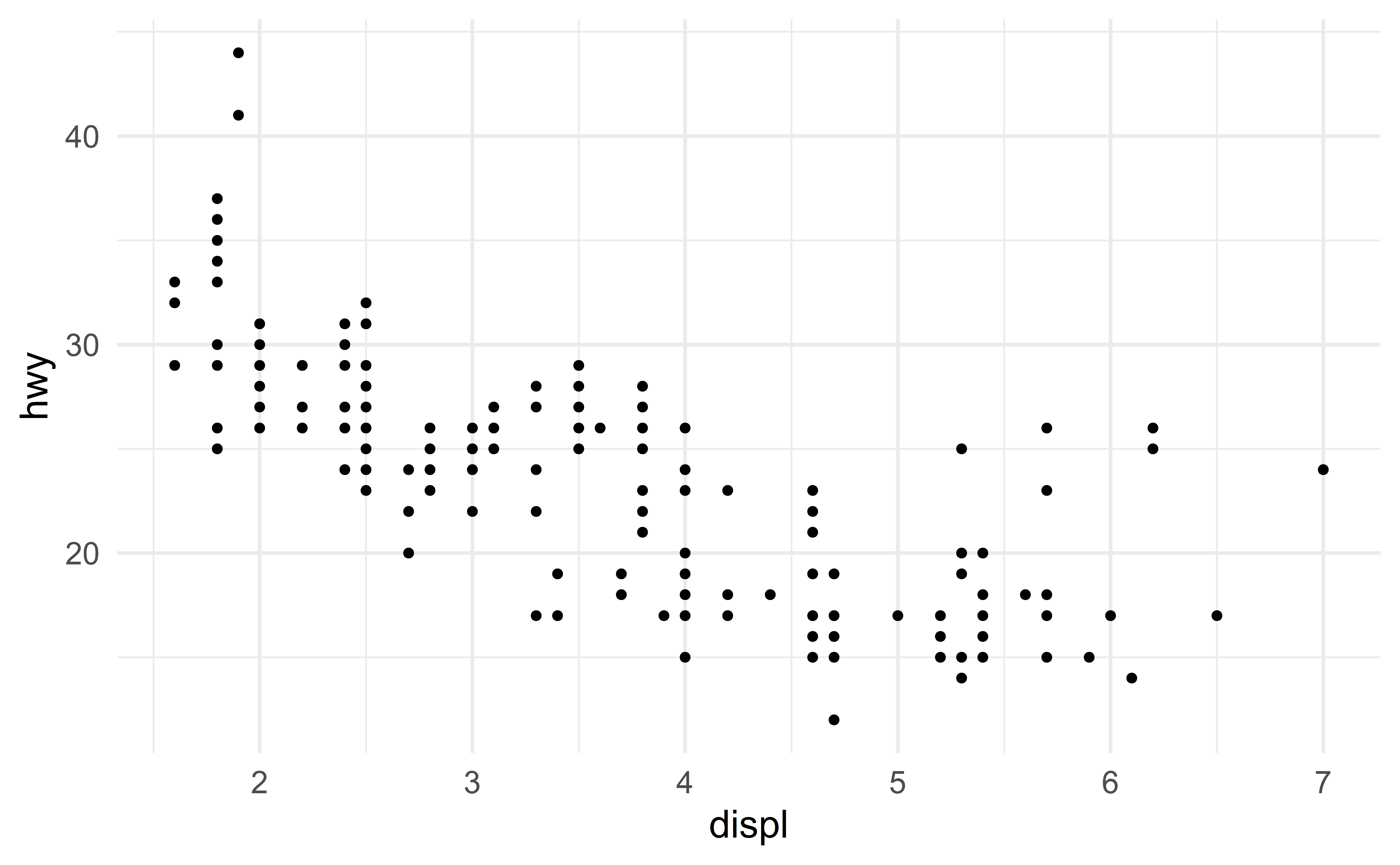
ggplot(d) +
  geom_point(aes(x = cty, y = hwy)) +
  geom_abline(intercept = 0.892, slope = 1.337, col = "red")

Reading `R` output

R can provide the results of a model in different formats.

m <- lm(hwy ~ cty, data = d)

Estimates only
Raw R output
Tidy R output


Call:
lm(formula = hwy ~ cty, data = d)

Coefficients:
(Intercept)          cty  
      0.892        1.337

Printing the model itself provides the least-square estimates. This is sufficient for now.

summary(m)


Call:
lm(formula = hwy ~ cty, data = d)

Residuals:
    Min      1Q  Median      3Q     Max 
-5.3408 -1.2790  0.0214  1.0338  4.0461 

Coefficients:
            Estimate Std. Error t value Pr(>|t|)    
(Intercept)  0.89204    0.46895   1.902   0.0584 .  
cty          1.33746    0.02697  49.585   <2e-16 ***
---
Signif. codes:  0 '***' 0.001 '**' 0.01 '*' 0.05 '.' 0.1 ' ' 1

Residual standard error: 1.752 on 232 degrees of freedom
Multiple R-squared:  0.9138,    Adjusted R-squared:  0.9134 
F-statistic:  2459 on 1 and 232 DF,  p-value: < 2.2e-16

This format contains information that will be useful when we do inference. It is, however, difficult to read.

summary(m) %>%
  tidy() %>%
  kable(digits = 2)

term	estimate	std.error	statistic	p.value
(Intercept)	0.89	0.47	1.90	0.06
cty	1.34	0.03	49.58	0.00

This format contains the information necessary for doing inference and is easy to read. This is the format used the textbook.

Exploring the model

The command augment from the R package broom gives us the residuals (.resid) and predictions (.fitted).

library(broom)
m <- lm(hwy ~ cty, data = d)
augment(m)[,1:4]

# A tibble: 234 x 4
     hwy   cty .fitted .resid
   <int> <int>   <dbl>  <dbl>
 1    29    18    25.0 4.03  
 2    29    21    29.0 0.0214
 3    31    20    27.6 3.36  
 4    30    21    29.0 1.02  
 5    26    16    22.3 3.71  
 6    26    18    25.0 1.03  
 7    27    18    25.0 2.03  
 8    26    18    25.0 1.03  
 9    25    16    22.3 2.71  
10    28    20    27.6 0.359 
# ... with 224 more rows

Group exercise - exploring a model

Consider the third observation in the sample. What is its

value of cty?
predicted value for hwy based on the model?
actual value for hwy?
residual?
Does the model over- or under-predict?

03:00

Intepreting the parameters

the intercept estimate \(\hat{\beta}_0\) is the prediction for a car with \(\text{cty} = 0\)
- meaningless in our case

the slope estimate \(\hat{\beta}_1\) is the increase in a our prediction for hwy for each additional unit of cty
- “for each additional unit of cty, we expect hwy to increase by 1.337”

Extrapolation

Stick to the range of the data
- if you extrapolate, do so with care, not like this.
The intercept will not always be meaningful

Group exercise - least-square estimates

Exercise 7.21

skip part c
start by fitting the model in R with the following command,

d <- openintro::coast_starlight
m <- lm(travel_time ~ dist, data = d)

05:00

Special case: categorical predictor

Let us create a binary predictor indicating if the car is from \(1999\).

d_binary <- mutate(d, year_binary = if_else(year == 1999, 1, 0))
head(select(d_binary, hwy, year, year_binary))

# A tibble: 6 x 3
    hwy  year year_binary
  <int> <int>       <dbl>
1    29  1999           1
2    29  1999           1
3    31  2008           0
4    30  2008           0
5    26  1999           1
6    26  1999           1

The variable year_binary takes the value \(1\) if the car is from \(1999\) and \(0\) otherwise.

m_binary <- lm(hwy ~ year_binary, data = d_binary)
m_binary


Call:
lm(formula = hwy ~ year_binary, data = d_binary)

Coefficients:
(Intercept)  year_binary  
   23.45299     -0.02564

The model equation is

\[ \text{hwy} \approx 23.46 - 0.026 \text{year_binary} \]

For a new car from \(1999\), the variable year_binary takes the value \(1\) and our prediction is

\[ \widehat{\text{hwy}} = 23.46 - 0.026*1 = 23.46 - 0.026 = 23.434 \]

While for a car that not from \(1999\), the variable year_binary takes the value \(0\) and our prediction is

\[ \widehat{\text{hwy}} = 23.46 - 0.026*0 = 23.46 - 0 = 23.46 \]

Model comparison

Alternative model

Let us fit an alternative model using engine size (disp) as a predictor

\[ \text{hwy} \approx \beta_0 + \beta_1 \text{displ} \]

ggplot(d) +
  geom_point(aes(displ, hwy))

The least-square estimates for the coefficients are

lm(hwy ~ displ, data = d)


Call:
lm(formula = hwy ~ displ, data = d)

Coefficients:
(Intercept)        displ  
     35.698       -3.531

Note that the slope coefficient is negative; which makes sense since we would expect cars with larger engines to be less efficient.

We now have two models. Which is the best?

We could start by looking at the residuals

Comparing residuals

m1 <- lm(hwy ~ cty, data = d)
m_augment <- augment(m1)
ggplot(m_augment) +
  geom_histogram(aes(.resid)) +
  xlim(-15, 15)

lm(hwy ~ displ, data = d) %>%
  augment %>%
  ggplot() +
  geom_histogram(aes(.resid)) +
  xlim(-15, 15)

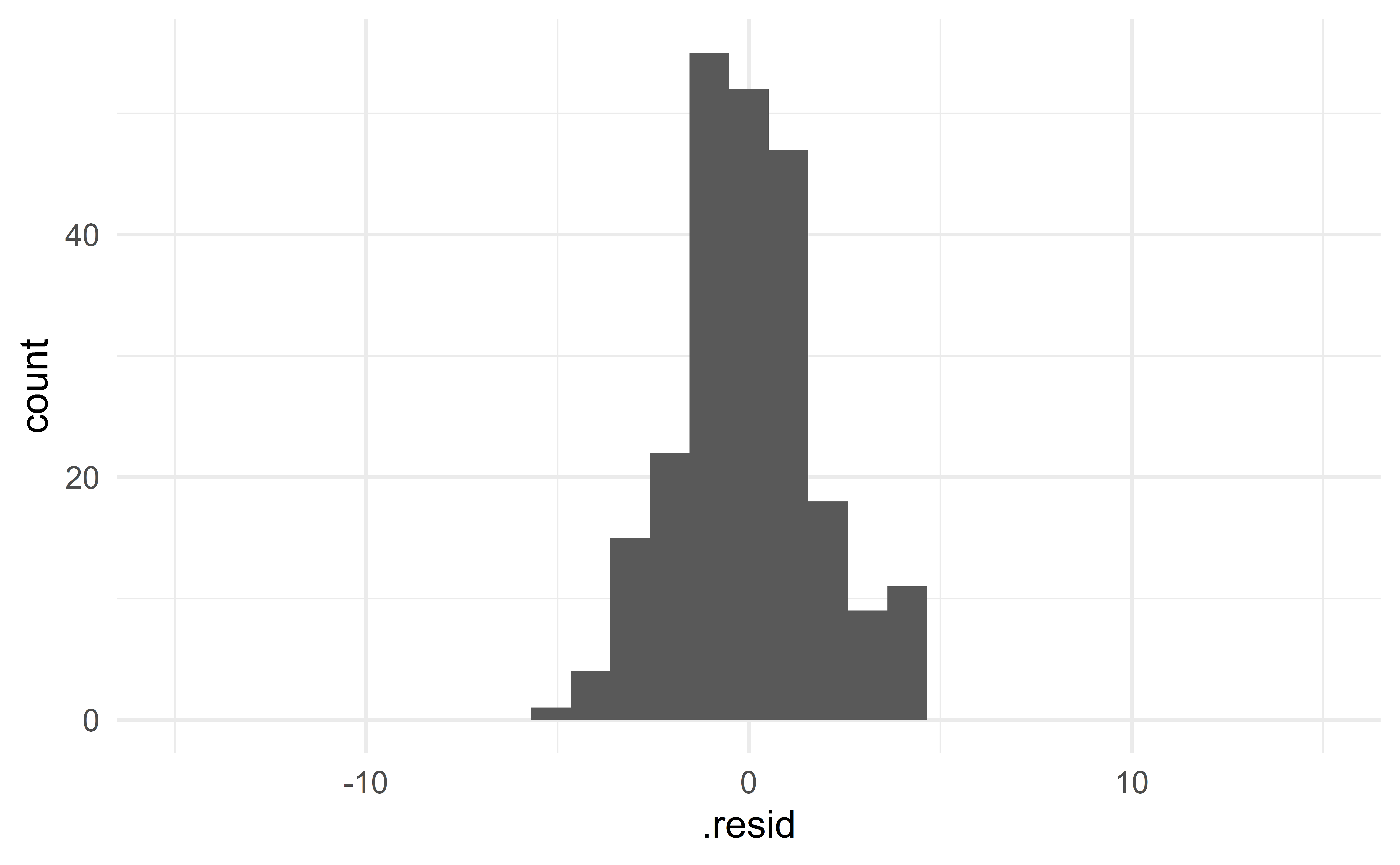
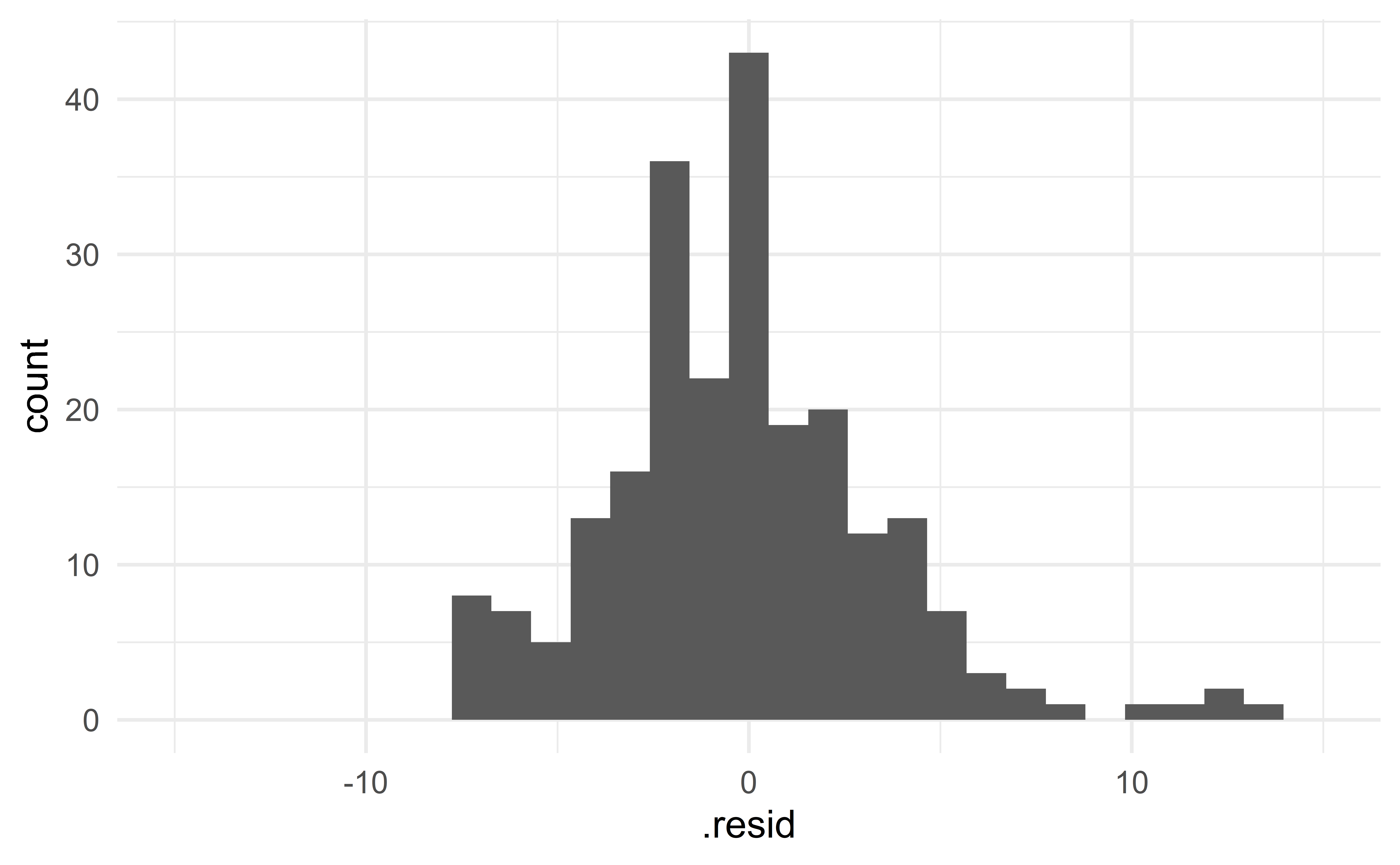
The first model seems to have smaller residuals.

\(\Rightarrow\) choose the first model!

Comparing models in a systematic way

But looking at a plot can be misleading

illusions
difficult to compare models with similar residuals

We need a more systematic approach for comparing models.

SSR

Instead of comparing histograms of residuals, we can compute the SSR (sum of squared residuals!)

\[\begin{align*} SSR & = r_1^2+r_2^2+\dots+r^2_n \\ & = (y_1 - \hat{y}_1)^2 + (y_2 - \hat{y}_2)^2 + \dots + (y_n - \hat{y}_n)^2 \end{align*}\]

small residuals will give a small SSR
large residuals will give a large SSR

\(\Rightarrow\) choose the model with the smaller SSR!

📋 The textbook uses the term SSE (sum of squared errors).

SSR of the first model:

m1 <- lm(hwy ~ cty, data = d)
m_augment <- augment(m1)
resid <- m_augment$.resid
sum(resid^2)

[1] 712.3599

SSR of the second model:

lm(hwy ~ displ, data = d) %>%
  augment %>% 
  .[[".resid"]] %>% 
  .^2 %>% 
  sum

[1] 3413.829

We opt for the first model (smaller SSR).

\(R^2\)

While the SSR is useful for comparing models, it can also be used to describe the goodness of fit of the model.

The SST (total sum of squares) is the sum of squared distance to the mean.

\[ SST = (y_1 - \bar{y})^2 + (y_2 - \bar{y})^2 + \dots + (y_n - \bar{y})^2 \]

It measures the total amount of variability in the data.

Remember the formula for SSR

\[ SSR = (y_1 - \hat{y}_1)^2 + (y_2 - \hat{y}_2)^2 + \dots + (y_n - \hat{y}_n)^2 \]

It measures the amount of variability in the data left unexplained by the model.

\(SST - SSR\) (total - residual) is therefore the amount of variation explained by the model:

\[ \text{data} = SST = (SST-SSR) + SSR = \text{model} + \text{residuals} \]

The statistic \(R^2\) measures the proportion of variation in the data that is explained by the model.

\[ \begin{align*} R^2 & = 1-\dfrac{SSR}{SST}\\ & = \dfrac{SST-SSR}{SST} \\ & = \dfrac{\text{var. explained by model}}{\text{total var.}} \end{align*} \]

Note that \(0\le R^2 \le 1\).

good model \(\Rightarrow\) small residuals \(\Rightarrow\) small SSR \(\Rightarrow\) large \(R^2\).
great model \(\Rightarrow\) tiny residuals \(\Rightarrow\) tiny SSR \(\Rightarrow\) \(R^2\) close to 1.
poor model \(\Rightarrow\) large residuals \(\Rightarrow\) SSR almost as large as SST \(\Rightarrow\) \(R^2\) close to 0.

Computing \(R^2\) in `R`

To compute \(R^2\) in R, simply use the command glance.

m1 <- lm(hwy ~ cty, data = d)
m_glance <- glance(m1)
m_glance$r.squared

[1] 0.9137752

lm(hwy ~ displ, data = d) %>% 
  glance %>% 
  .[["r.squared"]]

[1] 0.5867867

The model with cty as a predictor has a \(R^2\) value of \(0.914\), and the model that uses displ has a \(R^2\) of \(0.59\) (worse).

The first model is better!

Group exercise - Interpretation

Exercise 7.23
- fit the model in R; do you obtain the same estimates?
- do parts a-d
- compute the SST, SSR and \(R^2\) “by hand” in R (do not use glance). You can use the command augment to compute the residuals.

d <- usdata::county_2019
m <- lm(. . .)
m_augment <- augment(m)
SST <- ...

05:00

Outliers

Outliers in regression

Remember, in a boxplot, outliers are observations far from the bulk of the data

ggplot(d) +
  geom_boxplot(aes(hwy))

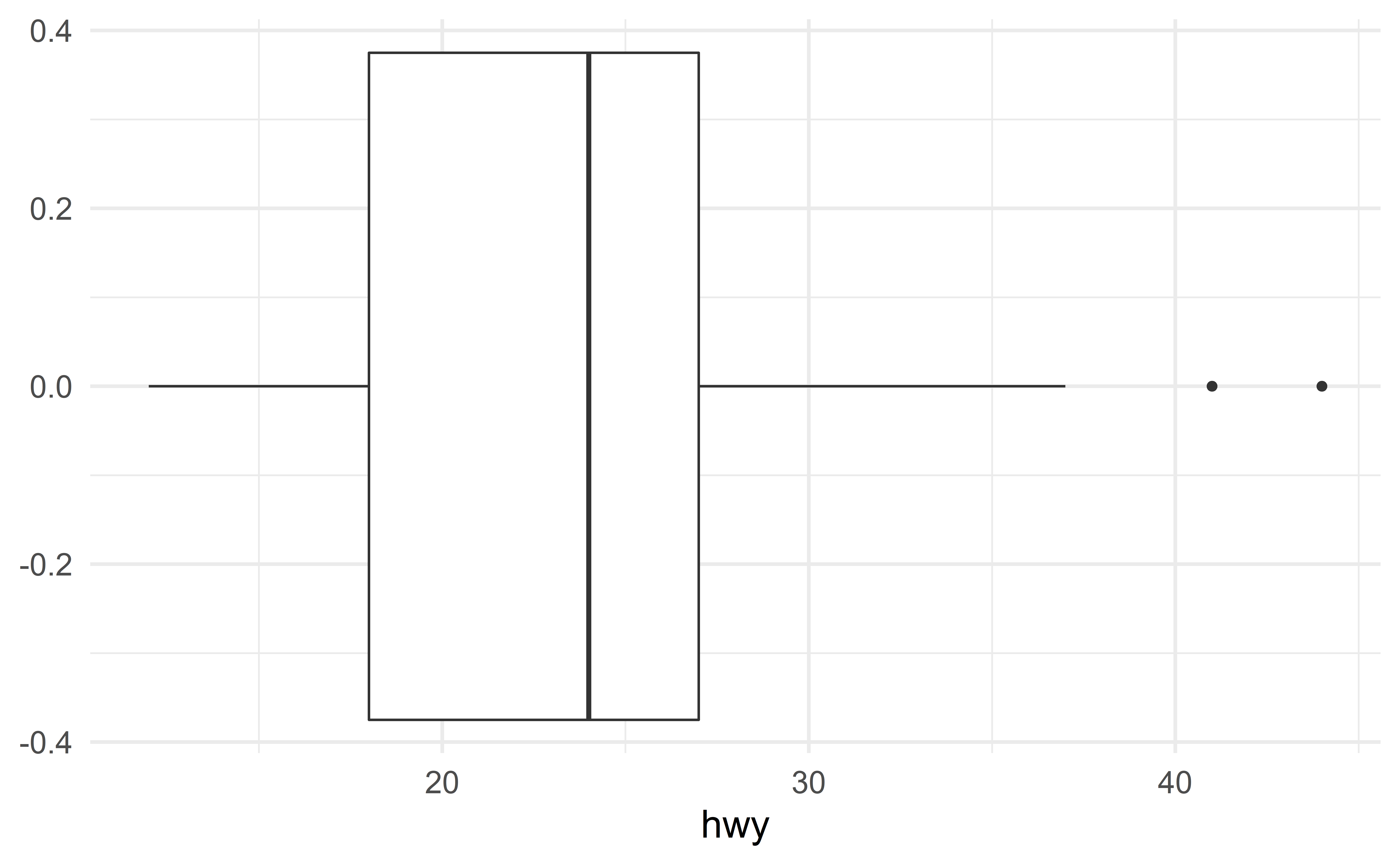
In the context of regression models, an outlier is an observation that falls far from the cloud of points

Identifying outliers

In the following scatterplot, we see two outliers

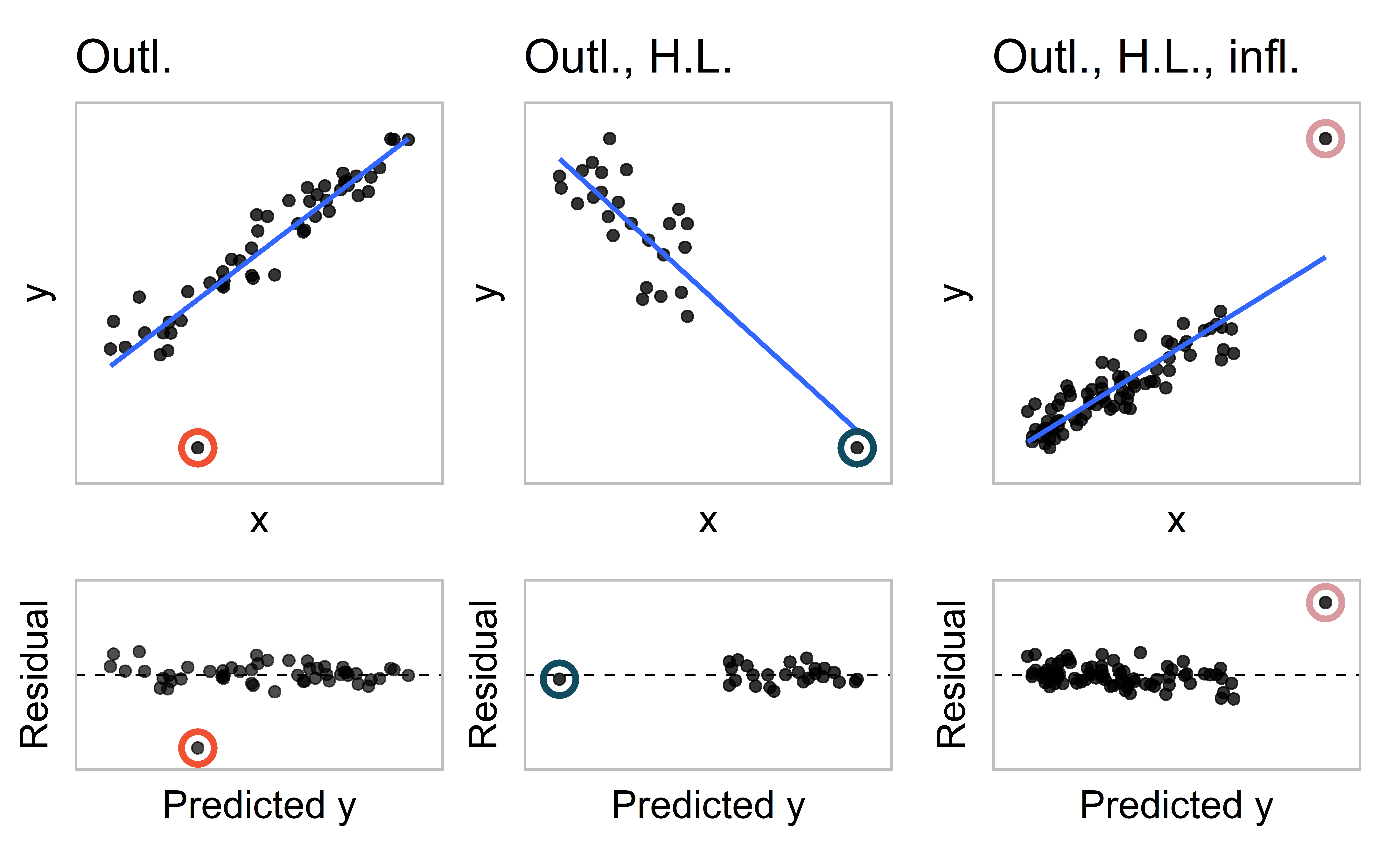
ggplot(d) +
  geom_point(aes(cty, hwy))

Group exercise - outlier in regression

Exercise 7.25

02:00

Outliers, leverage and influential points

outliers: observations that fall far from the cloud of points;
high leverage points: observations that fall horizontally away from the cloud of points;
influential points: observations that influence the slope of the regression line;

All influential points are high leverage points.
All leverage points are outliers.
(Venn Diagram)

Source: IMS

Group exercise - outlier

Exercise 7.27

03:00

Least-square estimates are not robust

In regression, outliers have the potential to highly influence the least-square estimates \(\hat{\beta}_0\) and \(\hat{\beta}_1\).

Warning

Least-square estimates are not robust to the presence of outliers.

Estimates that are robust include (not covered in this class)

least absolute deviation estimates, which minimize the SAR (sum of absolute residuals) instead of the SSR

\[ SAR = |e_1| + |e_2| + \dots + |e_n| \]

Bayesian estimates (STA360)

Impact of outliers

Let us contaminate the data with an outlier (cty \(=10\) and hwy \(=1000\))

d_contaminated <- select(d, cty, hwy) %>%
  add_row(cty = 40, hwy = 500) # add outlier
arrange(d_contaminated, desc(hwy)) %>% slice(1:5)

# A tibble: 5 x 2
    cty   hwy
  <dbl> <dbl>
1    40   500
2    33    44
3    35    44
4    29    41
5    28    37

…and compare the two regression models.

lm(hwy ~ cty, data = d)


Call:
lm(formula = hwy ~ cty, data = d)

Coefficients:
(Intercept)          cty  
      0.892        1.337

lm(hwy ~ cty, data = d_contaminated)


Call:
lm(formula = hwy ~ cty, data = d_contaminated)

Coefficients:
(Intercept)          cty  
    -33.841        3.498

The slope estimate has almost tripled!

ggplot(d_contaminated) +
  geom_point(aes(cty, hwy)) +
  geom_abline(intercept = -33.841, slope = 3.498, col = "purple")

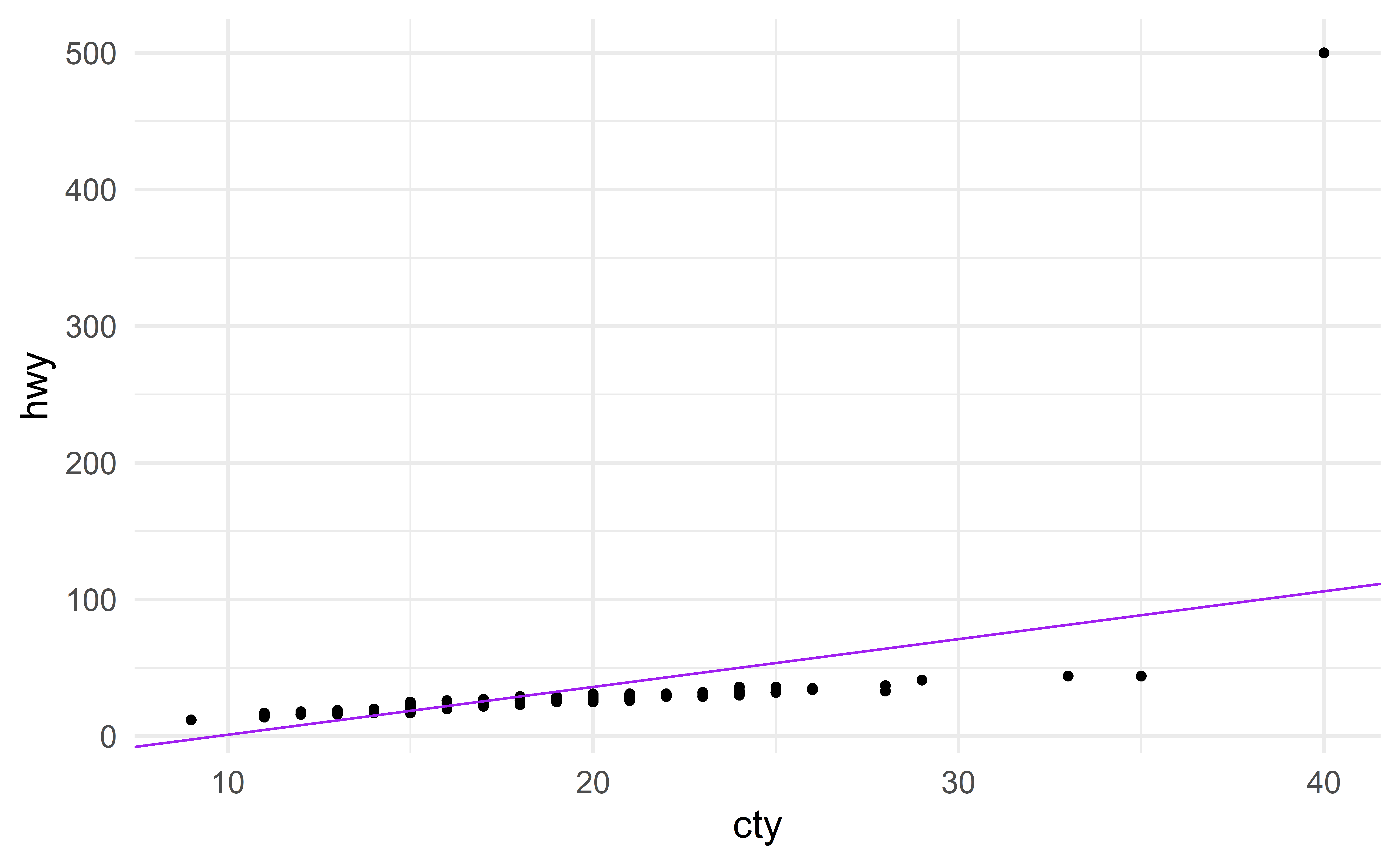
The regression line not longer fits the data well.

Statistics as an art - dealing with outliers

Dealing with outliers

Outliers can unduly influence parameter estimates. How to deal with an outlier depends on why the observation stands out. Outliers can either be

removed
corrected
ignored

Recap

simple linear regression model

\[ \text{hwy} \approx \beta_0 + \beta_1 \text{cty} \]

residuals
least-square estimates
parameter interpretation
model comparison with \(R^2\)
outliers

Simple Linear Regression Models

Welcome

Announcements

Recap of last lecture

Outline

Simple linear regression

Regression model

Simple regression

Simple linear regression

Parameters

Prediction

Linear association

Leat-square estimates

Residuals

Visualizing residuals

Residual plot

Assessing linearity with residual plots

Good estimates

Minimizing residuals

Why squaring the residuals?

Least-square estimates

Visualizing the least square regression line

Reading R output

Exploring the model

Intepreting the parameters

Special case: categorical predictor

Model comparison

Alternative model

Comparing residuals

Comparing models in a systematic way

SSR

\(R^2\)

Computing \(R^2\) in R

Outliers

Outliers in regression

Identifying outliers

Outliers, leverage and influential points

Least-square estimates are not robust

Impact of outliers

Statistics as an art - dealing with outliers

Recap

Recap

Reading `R` output

Computing \(R^2\) in `R`