Inference for regression

STA 101L - Summer I 2022

Raphael Morsomme

Welcome

Announcements – remaining deadlines

Homework
- 6 – tonight
- 7 – Monday, June 13
- 8 – Thursday, June 16
- 9 – Sunday, June 19 (no penalty for 24 hours – Monday, June 20)
- one free 24-hour deadline extension; lowest grade dropped
Inference project
- Presentation – Friday, June 17 (lab)
- Written report – Thursday, June 23

Announcements – inference project

Teams
Overview
2 data sets or topics before tomorrow’s lab
Leave lab with a data set

Recap

The normal distribution

One mean (case 3)
- CI via bootstrap

Two means (case 4)
- HT via simulation
- CI via bootstrap

Paired means (similar to one mean)
- HT via simulation
- CI via bootstrap
- Always pair!

Outline

Simple linear regression (case 5)
- HT via simulation
- CI via bootstrap

Simple linear regression

Setup

Simple linear regression: \(Y \approx \beta_0 + \beta_1 X\)

Population parameter: slope parameter \(\beta_1\)

Sample statistic: least-square estimate \(\hat{\beta}_1\)

Confidence interval: range of plausible values for \(\beta_1\)

Hypothesis test: is the response variable \(Y\) independent of the predictor \(X\)?

\(H_0:\beta_1 = 0\) (\(Y\) does not depend on \(X\))
\(H_a:\beta_1\neq0\)

Example – birth weight

set.seed(47)
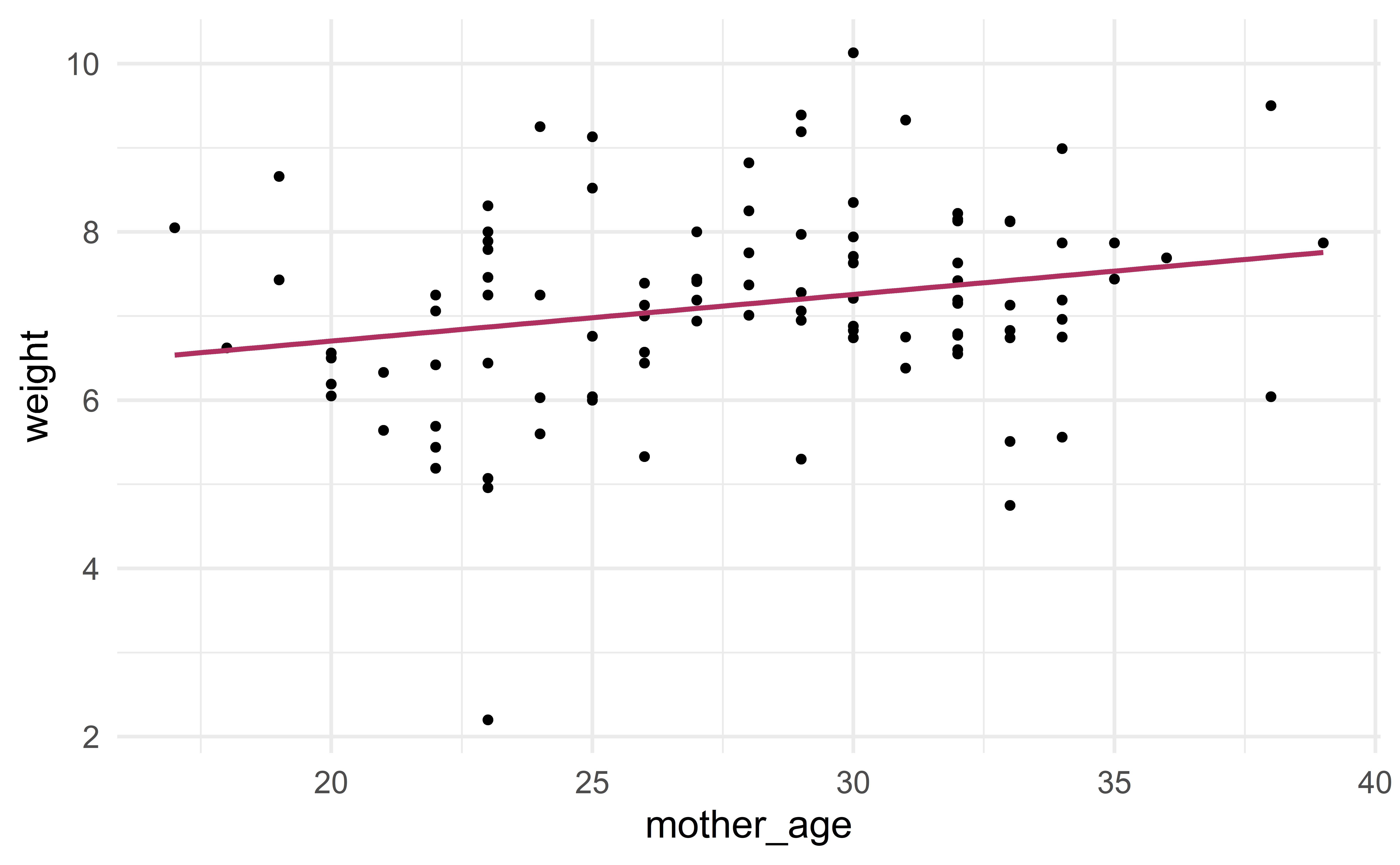
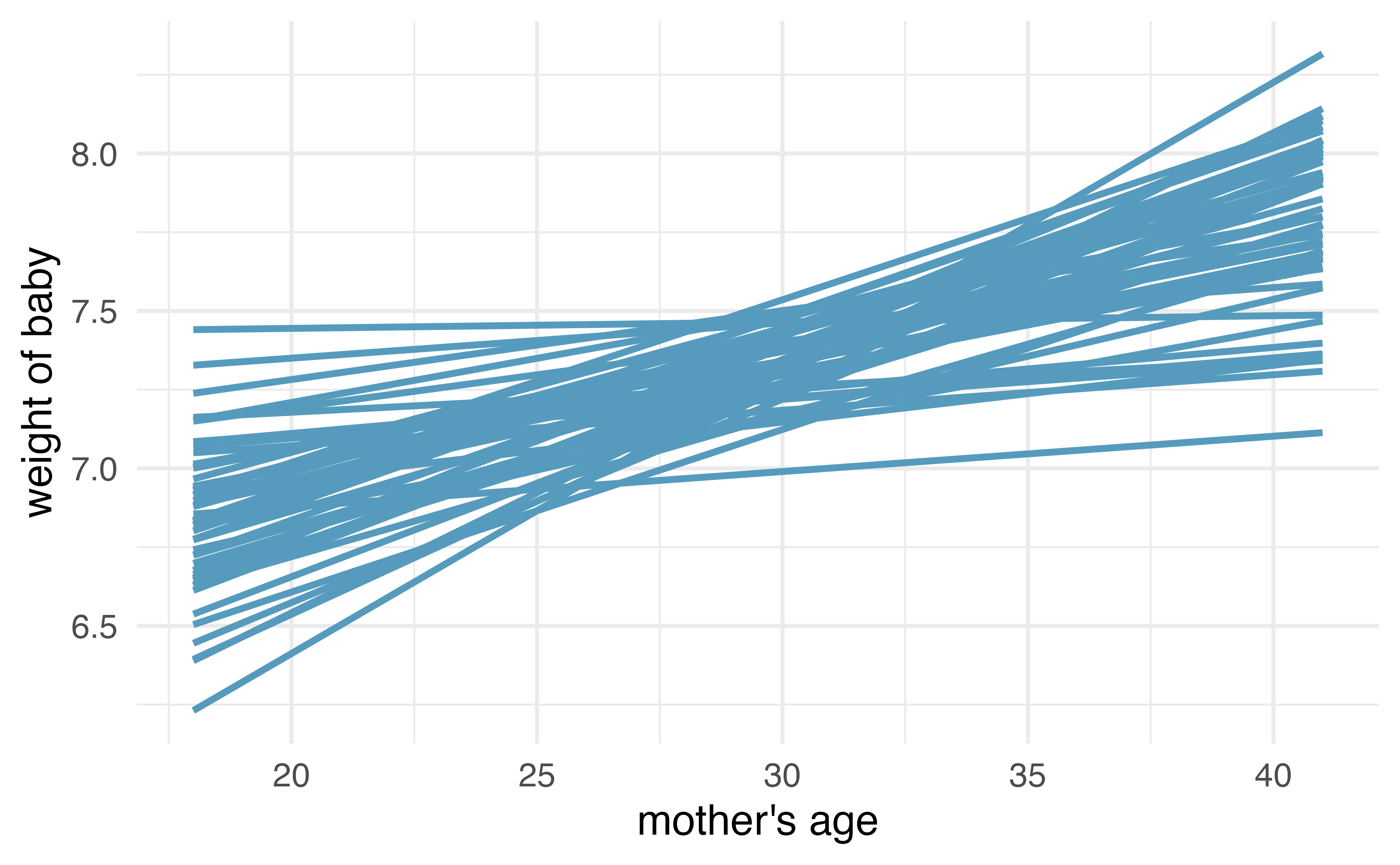
d <- openintro::births14 %>%
  sample_n(100) %>% # take a random sample of 100 births
  select(weight, mage) %>% # only keep the variables weight (newborn's weight) and mage (mother's age) 
  rename(mother_age = mage)
head(d)

# A tibble: 6 x 2
  weight mother_age
   <dbl>      <dbl>
1   6.94         27
2   9.19         29
3   7.39         26
4   8.82         28
5   7.87         35
6   9.39         29

Original data

ggplot(d, aes(x = mother_age, y = weight)) +
  geom_point() +
  geom_smooth(method = "lm", se = FALSE, col = "maroon") # regression line

Individual exercise - gut feeling

Do you intuitively feel that the pattern could be explained by chance alone?

01:00

Hypothesis test via simulation

Hypotheses and simulations

\(H_0:\beta_1=0\)

\(H_a:\beta_1\neq 0\)

Simulate many samples under \(H_0\) (the response variable is independent of the predictor).
Determine if the observed data could have plausibly arisen under \(H_0\).

Simulating under \(H_0\)

Under \(H_0\), there is no relation between the response and the predictor

\(\Rightarrow\) the newborn’s weight is independent of the mother’s age

\(\Rightarrow\) randomly re-assign the predictor independently of the response.

d_sim <- d %>% mutate(mother_age = sample(mother_age)) # shuffle the response
head(d)

# A tibble: 6 x 2
  weight mother_age
   <dbl>      <dbl>
1   6.94         27
2   9.19         29
3   7.39         26
4   8.82         28
5   7.87         35
6   9.39         29

head(d_sim)

# A tibble: 6 x 2
  weight mother_age
   <dbl>      <dbl>
1   6.94         23
2   9.19         23
3   7.39         23
4   8.82         22
5   7.87         30
6   9.39         29

Function for computing the test statistic

compute_beta_LS <- function(data){
  m     <- lm(weight ~ mother_age, data = data)
  coef  <- m$coefficients
  slope <- coef[["mother_age"]] 
  return(slope)
}
compute_beta_LS(d_sim)

[1] 0.03606311

For-loop for simulating under \(H_0\)

results <- tibble(stat_sim = numeric())
set.seed(1)
for(i in 1 : 10e3){ # 10,000 iterations
  d_sim    <- d %>% mutate(mother_age = sample(mother_age)) # simulate under H0
  stat_sim <- compute_beta_LS(d_sim) # statistic
  results  <- results %>% add_row(stat_sim)
}

Sampling distribution

stat_obs <- compute_beta_LS(d)
stat_obs

[1] 0.05542352

ggplot(results) + 
  geom_histogram(aes(stat_sim)) +
  geom_vline(xintercept = stat_obs, col = "maroon", size = 2)

p-value

Probability that \(\hat{\beta}_{1}^{sim}\ge \hat{\beta}^{obs}_1\) or \(\hat{\beta}_{1}^{sim}\le -\hat{\beta}^{obs}_1\).

p_value <- results %>%
  mutate(is_more_extreme = stat_sim >= stat_obs | stat_sim <= -stat_obs) %>%
  summarize(p_value = mean(is_more_extreme))
p_value

# A tibble: 1 x 1
  p_value
    <dbl>
1  0.0228

Using the usual significance level \(\alpha = 0.05\), we reject \(H_0\).

m <- lm(weight~mother_age, data = d)
broom::tidy(m)

# A tibble: 2 x 5
  term        estimate std.error statistic  p.value
  <chr>          <dbl>     <dbl>     <dbl>    <dbl>
1 (Intercept)   5.59      0.669       8.36 4.35e-13
2 mother_age    0.0554    0.0237      2.34 2.13e- 2

Group exercise - HT

Exercise 24.1 – in part c, refer to the output of the lm command (mathematical model)

Exercise 24.9 – in part c, refer to the output of the lm command (mathematical model)

03:00

Confidence interval via bootstrap

Bootstrap

sample_bootstrap <- function(data){ # same function as before
  n                <- nrow(data)
  sample_bootstrap <- slice_sample(data, n = n, replace = TRUE)
  return(sample_bootstrap)
}

set.seed(0)
sample_bootstrap(d)

# A tibble: 100 x 2
   weight mother_age
    <dbl>      <dbl>
 1   7.44         35
 2   6.83         30
 3   5.3          29
 4   6.94         27
 5   5.07         23
 6   6.03         24
 7   6.44         26
 8   7.44         35
 9   7.13         33
10   7.25         23
# ... with 90 more rows

Source: IMS

results <- tibble(stat_boot = numeric())
set.seed(0)
for(i in 1 : 5e3){ # 5,000 iterations
  d_boot    <- sample_bootstrap(d)     # bootstrap sample
  stat_boot <- compute_beta_LS(d_boot) # bootstrap statistic
  results   <- results %>% add_row(stat_boot) 
}

Source: IMS

Simulated slopes

ggplot(results) + 
  geom_histogram(aes(stat_boot)) + 
  geom_vline(xintercept = quantile(results$stat_boot, c(0.05, 0.95)), col = "gold1" , size = 2) + # 90% CI 
  geom_vline(xintercept = quantile(results$stat_boot, c(0.01, 0.99)), col = "maroon", size = 2) # 98% CI

CI and HT

quantile(results$stat_boot, c(0.05, 0.95)) # 90% CI (doesn't include 0)

        5%        95% 
0.01508696 0.09440465

quantile(results$stat_boot, c(0.01, 0.99)) # 98% CI (includes 0)

           1%           99% 
-0.0001734654  0.1117749557

Remember that the p-value is 0.023.

Two sides of the same coin

The 95% CI dos not include 0, but the 98% CI does. This indicates that 0 is a value plausible at the (usual) significance level \(\alpha=0.05\) but not at the more conservative significance level \(\alpha=0.02\). Again, this is exactly what the HT concluded.

Group exercise - CI

Exercise 24.3. Does the CI include 0? Does it agree with the HT?

Exercise 24.11. Does the CI include 0? Does it agree with the HT?

03:00

Recap

Simple linear regression (case 5)
- HT via simulation
- CI via bootstrap