library(tidyverse)
library(broom)rmd_demo
This document contains a few tips for working with RMD files. The source file has been sent by email.
Level-1 title (often too large)
Level-2 title (typically better than level-1)
You always want to start by loading the packages you will need.
The next step typically consists in downloading the data
d <- read_csv("https://rmorsomme.github.io/website/projects/training_set.csv")Rows: 1000 Columns: 16
-- Column specification --------------------------------------------------------
Delimiter: ","
chr (2): mother_diabetes_gestational, newborn_sex
dbl (13): newborn_birth_weight, month, mother_age, prenatal_care_starting_mo...
lgl (1): mother_risk_factor
i Use `spec()` to retrieve the full column specification for this data.
i Specify the column types or set `show_col_types = FALSE` to quiet this message.and then perhaps fitting a model.
m <- lm(mother_bmi ~ mother_weight_prepregnancy, data = d)
m
Call:
lm(formula = mother_bmi ~ mother_weight_prepregnancy, data = d)

Coefficients:
               (Intercept)  mother_weight_prepregnancy
                    2.6622                      0.1552
This is simply an illustration. In the project, you should not use mother_bmi as the response!
For the project, simply save the model you have selected in a RDATA file and send it to the instruction team.
save(m, file = "my_predictive_model.RDATA")
rm(m) # removes the object `m` from the environment
Once we have everybody’s model, we will use the following commands to load them into R and test them on new data.
load("my_predictive_model.RDATA")

new_data <- tibble(mother_weight_prepregnancy = 150) # new data
predict(m, new_data)
1
25.93563 We can use RMD to write mathematical expressions
To write a small mathematical expression, simply write it between $ signs.
For instance, \(x = 5 + 9\).
To write longer expression, use two $ signs.
\[ Y \approx \beta_0 + \beta_1 X_1 + \beta_2 X_2 \]
To write a word in a math equation, use \text{}
\[ \text{BMI} \approx \beta_0 + \beta_1 \text{weight} + \beta_3 X^2 \]
Running R code
You can run R code in R chunks:
5+5[1] 10You can also directly run R code in a paragraph as follows: using ` r 5+5`. For instance, the \(R^2\) value of model m is 0.882.
Learning more about RMD
Come to OH, ask questions during/after class.
Check the RMD cheatsheet or the longer reference guide.
Overall goal of the prediction project
two baseline models (simple and full) + 3 models that you construct
feature engineering + model selection
the outcome of that procedure should be a model that predicts the response variable reasonably well
please refer to the rubric
Missing values in the penguin dataset?
d <- palmerpenguins::penguins

filter(d,  is.na(body_mass_g)) # keeps the rows with a missing value for body_mass_g
# A tibble: 2 x 8
species island bill_length_mm bill_depth_mm flipper_length_~ body_mass_g sex
<fct> <fct> <dbl> <dbl> <int> <int> <fct>
1 Adelie Torge~ NA NA NA NA <NA>
2 Gentoo Biscoe NA NA NA NA <NA>
# ... with 1 more variable: year <int>filter(d, !is.na(body_mass_g)) # keeps the rows without a missing value for body_mass_g# A tibble: 342 x 8
species island bill_length_mm bill_depth_mm flipper_length_mm body_mass_g
<fct> <fct> <dbl> <dbl> <int> <int>
1 Adelie Torgersen 39.1 18.7 181 3750
2 Adelie Torgersen 39.5 17.4 186 3800
3 Adelie Torgersen 40.3 18 195 3250
4 Adelie Torgersen 36.7 19.3 193 3450
5 Adelie Torgersen 39.3 20.6 190 3650
6 Adelie Torgersen 38.9 17.8 181 3625
7 Adelie Torgersen 39.2 19.6 195 4675
8 Adelie Torgersen 34.1 18.1 193 3475
9 Adelie Torgersen 42 20.2 190 4250
10 Adelie Torgersen 37.8 17.1 186 3300
# ... with 332 more rows, and 2 more variables: sex <fct>, year <int>Conclusion
This is the end of the main body
Appendix
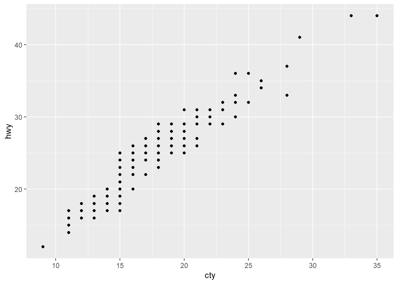
Figures should go here.
ggplot(mpg, aes(cty, hwy)) + geom_point()